Transcription of Discrete Fourier Transform (DFT)
1 Discrete Fourier Transform (DFT). Recall the DTFT: . X. X( ) = x(n)e j n. n= . DTFT is not suitable for DSP applications because In DSP, we are able to compute the spectrum only at specific Discrete values of , Any signal in any DSP application can be measured only in a finite number of points. A finite signal measured at N points: . 0, n < 0, x(n) = y(n), 0 n (N 1), 0, n N, . where y(n) are the measurements taken at N points. EE 524, Fall 2004, # 5 1. Sample the spectrum X( ) in frequency so that 2 . X(k) = X(k ), = = . N. N 1. j2 kn X. X(k) = x(n)e N DFT. n=0. The inverse DFT is given by: N 1. 1 X kn x(n) = X(k)ej2 N . N. k=0. 1. N. (N 1 ). 1 X X. j2 km j2 kn x(n) = x(m)e N e N. N m=0. k=0. 1 1. N. ( N. ). X 1 X. j2 . k(m n). = x(m) e N = x(n). m=0. N. k=0. | {z }. (m n). EE 524, Fall 2004, # 5 2. The DFT pair: N 1. X kn X(k) = x(n)e j2 N analysis n=0.
2 N 1. 1 X j2 kn x(n) = X(k)e N synthesis. N. k=0. Alternative formulation: N 1. X 2 . X(k) = x(n)W kn W = e j N. n=0. N 1. 1 X. x(n) = X(k)W kn. N. k=0. EE 524, Fall 2004, # 5 3. EE 524, Fall 2004, # 5 4. Periodicity of DFT Spectrum N 1. X (k+N )n j2 . X(k + N ) = x(n)e N. n=0. 1. N. ! j2 kn X. = x(n)e N e j2 n n=0. = X(k)e j2 n = X(k) = . the DFT spectrum is periodic with period N (which is expected, since the DTFT spectrum is periodic as well, but with period 2 ). Example: DFT of a rectangular pulse: . 1, 0 n (N 1), x(n) =. 0, otherwise. N 1. X kn X(k) = e j2 N = N (k) = . n=0. the rectangular pulse is interpreted by the DFT as a spectral line at frequency = 0. EE 524, Fall 2004, # 5 5. DFT and DTFT of a rectangular pulse (N=5). EE 524, Fall 2004, # 5 6. Zero Padding What happens with the DFT of this rectangular pulse if we increase N by zero padding: {y(n)} = {x(0).}
3 , x(M 1), 0, .. , 0} }, | 0,{z N M positions where x(0) = = x(M 1) = 1. Hence, DFT is N 1 M 1. j2 kn j2 kn X X. Y (k) = y(n)e N = y(n)e N. n=0 n=0. sin( kM. N ) j . k(M 1). = e N . sin( Nk ). EE 524, Fall 2004, # 5 7. DFT and DTFT of a Rectangular Pulse with Zero Padding (N = 10, M = 5). Remarks: Zero padding of analyzed sequence results in approximating its DTFT better, Zero padding cannot improve the resolution of spectral components, because the resolution is proportional to 1/M rather than 1/N , Zero padding is very important for fast DFT implementation (FFT). EE 524, Fall 2004, # 5 8. Matrix Formulation of DFT. Introduce the N 1 vectors . x(0) X(0). x(1) X(1) . x= .. , X= .. x(N 1) X(N 1). and the N N matrix . 0 0 0 0. W W W W.. W0 W1 W2 W N 1 .. W= . W0 W2 W4 W 2(N 1) .. (N 1)2. W 0 W N 1 W 2(N 1) W. DFT in a matrix form: X = Wx.
4 Result: Inverse DFT is given by 1 H. x= W X, N. EE 524, Fall 2004, # 5 9. which follows easily by checking W H W = WW H = N I, where I denotes the identity matrix. Hermitian transpose: xH = (xT ) = [x(1) , x(2) , .. , x(N ) ]. Also, denotes complex conjugation. Frequency Interval/Resolution: DFT's frequency resolution 1. Fres [Hz]. NT. and covered frequency interval 1. F = N Fres = = Fs [Hz]. T. Frequency resolution is determined only by the length of the observation interval, whereas the frequency interval is determined by the length of sampling interval. Thus Increase sampling rate = expand frequency interval, Increase observation time = improve frequency resolution. Question: Does zero padding alter the frequency resolution? EE 524, Fall 2004, # 5 10. Answer: No, because resolution is determined by the length of observation interval, and zero padding does not increase this length.
5 Example (DFT Resolution): Two complex exponentials with two close frequencies F1 = 10 Hz and F2 = 12 Hz sampled with the sampling interval T = seconds. Consider various data lengths N = 10, 15, 30, 100 with zero padding to 512. points. DFT with N = 10 and zero padding to 512 points. Not resolved: F2 F1 = 2 Hz < 1/(N T ) = 5 Hz. EE 524, Fall 2004, # 5 11. DFT with N = 15 and zero padding to 512 points. Not resolved: F2 F1 = 2 Hz < 1/(N T ) . Hz. DFT with N = 30 and zero padding to 512 points. Resolved: F2 F1 = 2 Hz > 1/(N T ) Hz. EE 524, Fall 2004, # 5 12. DFT with N = 100 and zero padding to 512. points. Resolved: F2 F1 = 2 Hz > 1/(N T ) =. Hz. EE 524, Fall 2004, # 5 13. DFT Interpretation Using Discrete Fourier Series Construct a periodic sequence by periodic repetition of x(n). every N samples: x(n)} = {.. , x(0), .. , x(N 1), x(0).
6 , x(N 1), ..}. {e | {z } | {z }. {x(n)} {x(n)}. The Discrete version of the Fourier Series can be written as X. j2 kn 1 X e j2 kn 1 X e x e(n) = Xk e N = X(k)e N = X(k)W kn, N N. k k k where X(k). e = N Xk . Note that, for integer values of m, we have (k+mN )n kn j2 kn W =e N =e j2 N = W (k+mN )n. As a result, the summation in the Discrete Fourier Series (DFS). should contain only N terms: N 1. 1 X e j2 kn x e(n) = X(k)e N DFS. N. k=0. EE 524, Fall 2004, # 5 14. Inverse DFS. The DFS coefficients are given by N 1. X kn X(k). e = e(n)e j2 N. x inverse DFS. n=0. Proof.. N 1 N 1 N 1. X. j2 kn X 1 X e j2 pn . j2 kn x e(n)e N = X(p)e N e N. N . n=0 n=0 p=0. 1 1. N. ( N. ). X 1 X. j2 . (p k)n = X(p). e e N = X(k). e p=0. N n=0. | {z }. (p k). 2. The DFS coefficients are given by N 1. X kn X(k). e = e(n)e j2 N. x analysis, n=0. N 1. 1 X e j2 kn x e(n) = X(k)e N synthesis.
7 N. k=0. EE 524, Fall 2004, # 5 15. DFS and DFT pairs are identical, except that DFT is applied to finite sequence x(n), DFS is applied to periodic sequence x e(n). Conventional (continuous-time) FS vs. DFS. CFS represents a continuous periodic signal using an infinite number of complex exponentials, whereas DFS represents a Discrete periodic signal using a finite number of complex exponentials. EE 524, Fall 2004, # 5 16. DFT: Properties Linearity Circular shift of a sequence: if X(k) = DFT {x(n)} then km X(k)e j2 N = DFT {x((n m) mod N )}. Also if x(n) = DFT 1{X(k)} then km x((n m) mod N ) = DFT 1{X(k)e j2 N }. where the operation mod N denotes the periodic extension x e(n) of the signal x(n): x e(n) = x(n mod N ). EE 524, Fall 2004, # 5 17. DFT: Circular Shift N. X 1. x((n m)modN )W kn n=0. N. X 1. = W km x((n m)modN )W k(n m). n=0. EE 524, Fall 2004, # 5 18.
8 N. X 1. = W km x((n m)modN )W k(n m)modN. n=0. = W kmX(k), where we use the facts that W k(lmodN ) = W kl and that the order of summation in DFT does not change its result. Similarly, if X(k) = DFT {x(n)}, then j2 mn X((k m)modN ) = DFT {x(n)e N }. DFT: Parseval's Theorem N 1 N 1. X 1 X. x(n)y (n) = X(k)Y (k). n=0. N. k=0. Using the matrix formulation of the DFT, we obtain H . 1 H 1 H. yH x = W Y W Y. N N. 1 H H 1 H. = Y W W } X = Y X. N2 | {z NI. N. EE 524, Fall 2004, # 5 19. DFT: Circular Convolution If X(k) = DFT {x(n)} and Y (k) = DFT {y(n)}, then X(k)Y (k) = DFT {{x(n)} ~ {y(n)}}. Here, ~ stands for circular convolution defined by N. X 1. {x(n)} ~ {y(n)} = x(m)y((n m) mod N ). m=0. DFT {{x(n)} ~ {y(n)}}. N 1 h i X PN 1 kn = m=0 x(m)y((n m) mod N ) W. n=0 | {z }. {x(n)}~{y(n)}. N 1 h i X PN 1. = n=0 y((n m) mod N )W kn x(m). m=0 | {z }.
9 Y (k)W km N. X 1. = Y (k) x(m)W km = X(k)Y (k). |m=0 {z }. X(k). EE 524, Fall 2004, # 5 20.