Transcription of DiscreteTimeControlSystems - ETH Z
1 Discrete Time Control SystemsLino GuzzellaSpring 20130-01 Lecture IntroductionInherently Discrete-Time Systems, example bank accountBank account, interest ratesr+>0 for positive,r >0 for negativebalancesx(k+ 1) = (1 +r+)x(k) +u(k), x(k)>0(1 +r )x(k) +u(k), x(k)<0(1)wherex(k) is the account s balance at timekandu(k) is theamount of money that is deposited to (u(k)>0) or withdrawn from(u(k)<0) the general such systems are described by a difference equation of theformx(k+ 1) =f(x(k), u(k)), x(k) n, u(k) m, f: n m n(2)with which an output equation of the formy(k) =g(x(k), u(k)), y(k) p, g: n m p(3)is often will learn how continuous-time systems can be transformed to aform similar to that that there is a fundamental difference between inherentlydiscrete time systems and such approximations: for the former thereis no meaningful interpretation of the system behavior in between thediscrete time instancesk={1,2.}
2 }, while the latter have a clearlydefined behavior also between two sampling Control SystemsMost important case: continuous-time systems controlled by a digitalcomputer with interfaces ( Discrete-Time Control and DigitalControl synonyms).Such a discrete-time control system consists of four major parts:1 ThePlantwhich is a continuous-time dynamic TheAnalog-to-Digital Converter(ADC).3 TheController( P), a microprocessor with a real-time TheDigital-to-Analog Converter(DAC) .3+ r(t)e(t)ADC PDACu(t)Planty(t)??4 The signalsy,e, anduare continuous-time variables. The variablesentering and exiting the microprocessor (block P) aresampled, ,the ADC is an idealizedsamplere(k) =e(k T),(4)The constant parameterTis thesampling output of the block P is again only defined at certain elements transform this variable into a continuous-time Holds(ZOH)u(t) =u(k T) t [k T,(k+ 1) T)(5)Higher-order holds available but seldom challenge: loop contains both continuous-time anddiscrete-time parts.]
3 Two analysis approaches possible: The analysis is carried out in the continuous-time domain, andthe discrete-time part has to be described by a continuous-timesystem with the input at point 3 and the output at point 2. The analysis is carried out in the discrete-time domain, andthecontinuous-time part has to be described by a discrete-timesystem with the input at point 1 and the output at point two approaches are not equivalent. Obviously, the first one ismore powerful since it will provide insights into the closed-loopsystem behavior for all timest. The second one will only yieldinformation at the discrete time instancesk T.
4 Accordingly, it is tobe expected that the second approach is easier to follow and thisconjecture will be confirmed (t)P(s)y(t) +r(t)e(t)34e(k)C(z)u(k)ZOH7 The output signal of the planty(t) is a function of the plant s inputu(t), a relation which may be described, for instance, by ordinarydifferential equations (in the finite dimensional case) or bytransferfunctionsP(s) (in the linear case).Outputu(k) of the discrete controllerC(z) depends on its inpute(k)in a recursive wayu(k) =f(e(k), e(k 1), .. , e(k n), u(k 1), u(k 2), .. , u(k n)) (6)For a linear controller, a frequency domain representationwill bederived (C(z)).8 The microprocessor performs these calculations once everysamplinginterval.
5 Important aspects of this part are the synchronization andthe computation delays (see folllowing Figure). Typically, theprogramming is done in a high-level computer language ( C isoften used). Hardware drivers provided by the manufacturers of theADC and rapid prototyping control hardware/software systems are are very convenient to test control algorithms becausetheydovetail with Matlab/Simulink. For series applications such systemsare too systemrepeatwait for interruptdata inputcompute controller outputupdate shift registersdata outputterminate taskuntil doneshut down systemA)interrupttimetimetimek+ 1k+ 1k+ 1 AAAAAAAAADDDDDDDDDCCCCCCCCCkkk =TB)C)10In all cases additional delays arise.
6 They may be added to theplantduring the controller design process, , ifP(s) is the true plant, thedesign process is carried out for the fictitious plante s P(s).Unfortunately, the delay will not be constant in cases A) and B)(no real-time operating system can guarantee that). In order to copewith that the controller will have to have a sufficient robustnessmargin (in this case phase margin). Approach C) shows how to avoidvarying computation delays by artificially delaying the output untilthe next interrupt stimulus arrives. This event will be strictlysynchronous such that in this case constant delays result. Thefictitious plant in this case will bee T s P(s).
7 11P(s)continuous-timesynthesisC(s)emulat ionT small B eC(z)C(z)discrete-timesynthesisP(z) A T large ZOH12 Organization of this TextChapter 2: emulation techniques (following the path B ), workswell when the sampling times are much smaller than the relevanttime constants of the system. No guarantee that stability orrobustness properties are invariant to the 3: main properties of the sample-and-hold procedure, ,use continuous-time methods to describe the main effects of thesampling and holding 4: mathematical description of discrete time signals andsystems. The Ztransformation (the analog of the Laplacetransformation), transformation of continuous-time systems todiscrete-time systems and stability 5: synthesis of control systems directly in the discrete-timedomain (path A ), classical (loop shaping, root-locus,etc.)
8 And modern methods (LQR, LQG, etc.), dead-beat, Lecture Emulation MethodsIntroductionIn this chapter theemulation approachwill be presented. First thekey idea is introduced using analogies from the numerical integrationof differential equations. As a by-product a shift operatorzwill beintroduced using informal arguments. Some first system stabilityresults can be obtained with that. The most useful emulationmethods are then introduced and some extensions are shown whichimprove the closed-loop system behavior. The chapter closes with adiscussion of the assumptions under which this approach isrecommended and what limitations have to be IdeasStarting point: PI controller, in the time domain defined byu(t) =kp e(t) +1 TiZt0e( ) d (7)and in the frequency domain byU(s) =kp 1 +1Ti s E(s)(8)16If such a controller is to be realized using a digital computer, theproportional part does not pose any problems.
9 The integratorrequires more attention. The simplest approach is to approximate itby Euler s forward rule (initial conditionq(0) = 0 is assumed)q(k T) =Zk T0e( ) d k 1Xi=0e(i T) T(9)For sufficiently smallTthis approximation yields a controller whichproduces a closed-loop behavior similar to the one observedincontinuous a delay-free (the delay can be included in the plant dynamics) andrecursive formulation the controller (7) can therefore beapproximated in discrete time byu(k T) =kp he(k T) +1Ti q(k T)i,q(k T+T) =q(k T) +e(k T) T(10)In order to simplify the reasoning below two definitions are useful: The notationx(k) is adopted to denote the value of the variablexat timek T.
10 The operatorzis used to denote a forward shift by one samplinginterval, ,z x(k) is equal tox(k+ 1).The shift operatorzis analogous to the Heavyside operators( differentiation ). The analogy can be carried further, , thebackward shift operation is denoted byz 1withz 1 x(k) =x(k 1).18 The operatorzcan be used to solve linear difference equationsy(k+n)+an 1 y(k+n 1)+..+a0 y(k) =bn u(k+n)+..+b0 u(k)(11)which are transformed toy(k)+z 1 an 1 y(k)+..+z n a0 y(k) =bn u(k)+..+z n b0 u(k)(12)and thereforey(k) =bn+z 1 bn 1+..+z n b01 +z 1 an 1+..+z n a0 u(k)(13)Apply this to the problem of approximating the PI controlleru(k) =kp 1 +TTi (z 1) e(k)(14)Therefores z 1T(15)19 The key idea of all emulation approaches is now to use thesubstitution (15) (or a similar one) to transform a givencontinuous-time controller transfer functionC(s) into a discrete-timetransfer functionC(z), ,C(z) C(s)|s=z 1T(16)and to use the shift properties of the variablezto derive a differencerecursion for the controller outputu(k).