Transcription of Dummy-Variable Regression
1 7 Dummy-VariableRegressionOne of the serious limitations of multiple- Regression analysis, as presented in Chapters 5and 6, is that it accommodates only quantitative response and explanatory variables. In thischapter and the next, I will explain how qualitative explanatory variables, calledfactors, can beincorporated into a linear current chapter begins with an explanation of how adummy-variable regressorcan becoded to represent adichotomous( , two-category) factor. I proceed to show how a set of dummyregressors can be employed to represent apolytomous(many-category) factor.
2 I next describehow interactions between quantitative and qualitative explanatory variables can be represented indummy- Regression models and how to summarize models that incorporate interactions. Finally,I explain why it does not make sense to standardize Dummy-Variable and interaction A Dichotomous FactorLet us consider the simplest case: one dichotomous factor and one quantitative explanatoryvariable. As in the two previous chapters, assume that relationships areadditive that is, that thepartial effect of each explanatory variable is the same regardless of the specific value at whichthe other explanatory variable is held constant.
3 As well, suppose that the other assumptions ofthe Regression model hold: The errors are independent and normally distributed, with zero meansand constant general motivation for including a factor in a Regression is essentially the same as for includ-ing an additional quantitative explanatory variable: (1) to account more fully for the responsevariable, by making the errors smaller, and (2) even more important, to avoid a biased assess-ment of the impact of an explanatory variable, as a consequence of omitting another explanatoryvariable that is related to concreteness, suppose that we are interested in investigating the relationship betweeneducation and income among women and men.
4 Figure (a) and (b) represents two small (ide-alized) populations. In both cases, the within- gender regressions of income on education areparallel. Parallel regressions imply additive effects of education and gender on income: Holdingeducation constant, the effect of gender is the vertical distance between the two regressionlines, which for parallel lines is everywhere the same. Likewise, holding gender constant,the effect of education is captured by the within- gender education slope, which for parallellines is the same for men and Figure (a), the explanatory variables gender and education are unrelated to each other:Women and men have identical distributions of education scores (as can been seen by projectingthe points onto the horizontal axis).
5 In this circumstance, if we ignore gender and regress incomeon education alone, we obtain the same slope as is produced by the separate within-gender1 Chapter 14 deals with will consider nonparallel within-group regressions in Section A Dichotomous Factor121(a)Education(b)EducationMenWome nIncomeIncomeMenWomenFigure data representing the relationship between income and education forpopulations of men (filled circles) and women (open circles). In (a), there is norelationship between education and gender ; in (b), women have a higher averagelevel of education than men.
6 In both (a) and (b), the within- gender ( , partial)regressions (solid lines) are parallel. In each graph, the overall ( , marginal) Regression of income on education (ignoring gender ) is given by the broken Because women have lower incomes than men of equal education, however, byignoring gender we inflate the size of the situation depicted in Figure (b) is importantly different. Here, gender and education arerelated, and therefore if we regress income on education alone, we arrive at a biased assessmentof the effect of education on income.
7 Because women have a higher average level of educationthan men, and because for a given level of education women s incomes are lower, on average,than men s, the overall Regression of income on education has anegativeslope even though thewithin- gender regressions have light of these considerations, we might proceed to partition our sample by gender and performseparate regressions for women and men. This approach is reasonable, but it has its limitations:Fitting separate regressions makes it difficult to estimate and test for gender differences in , if we can reasonably assume parallel regressions for women and men, we can moreefficiently estimate the common education slope by pooling sample data drawn from both particular, if the usual assumptions of the Regression model hold, then it is desirable to fit thecommon-slope model by least way of formulating the common-slope model isYi= + Xi+ Di+ i( )
8 WhereD, called adummy-variable regressoror anindicator variable, is coded 1 for men and 0for women:Di={1for men0for women3 That marginal and partial relationships can differ in sign is calledSimpson s paradox(Simpson, 1951). Here, themarginal relationship between income and education is negative, while the partial relationship, controlling for gender , 7. Dummy-Variable RegressionXY0 + 1 1 D = 1D = 0 Figure additive Dummy-Variable Regression model. The line labeledD=1 is for men;the line labeledD=0 is for , for women the model becomesYi= + Xi+ (0)+ i= + Xi+ iand for menYi= + Xi+ (1)+ i=( + )+ Xi+ iThese Regression equations are graphed in Figure is our initial encounter with an idea that is fundamental to many linear models: the dis-tinction betweenexplanatory ,genderis a qualitative explanatoryvariable ( , a factor), with categoriesmaleandfemale.}
9 The dummy variableDis a regressor,representing the factor gender . In contrast, the quantitative explanatory variableeducationandthe regressorXare one and the same. Were we to transform education, however, prior to enteringit into the Regression equation say, by taking logs then there would be a distinction betweenthe explanatory variable (education) and the regressor (log education). In subsequent sections ofthis chapter, it will transpire that an explanatory variable can give rise to several regressors andthat some regressors are functions of more than one explanatory to Equation and Figure , the coefficient for the dummy regressor givesthe difference in intercepts for the two Regression lines.
10 Moreover, because the within-genderregression lines are parallel, also represents the constant vertical separation between the lines,and it may, therefore, be interpreted as the expected income advantage accruing to men wheneducation is held constant. If men weredisadvantaged relative to women with the same level ofeducation, then would benegative. The coefficient gives the intercept for women, for whomD=0; and is the common within- gender education reveals the fundamental geometric trick underlying the coding of a dummy regres-sor: We are, in fact, fitting a Regression plane to the data, but the dummy regressorDis defined onlyat the values 0 and 1.