Transcription of ECON 600 Lecture 3: Profit Maximization
1 ECON 600 Lecture 3: Profit Maximization I. The Concept of Profit Maximization Profit is defined as total revenue minus total cost. = TR TC (We use to stand for Profit because we use P for something else: price.) Total revenue simply means the total amount of money that the firm receives from sales of its product or other sources. Total cost means the cost of all factors of production. But and this is crucial we have to think in terms of opportunity cost, not just explicit monetary payments. If the owner of the business also works there, we must include the value of his time.
2 If the firm owns machines or land, we must include the payments those factors could have earned if the firm had chosen to rent them out instead of using them. If only explicit monetary costs are considered, we get accounting Profit . But to find economic Profit , we need to take into account the opportunity cost, implicit or explicit of all resources employed. The main constraints faced by the firm are: technology, as summarized in the cost curves of the last Lecture ; the prices of factors of production, also taken into account by the cost curves; and the demand for its product.
3 II. Demand Curve Facing the Firm The firm s demand curve tells how much consumers will buy at each price from a particular firm. (This is distinguished from other kinds of demand curve, such as the market demand curve, which shows how much consumers will buy at each price from all firms put together.) The shape of the firm s demand curve is related to the degree of competition in the market. Loosely speaking, more competition causes the firm s demand curve to be more elastic (flatter), because consumers can respond to price increases by shifting their purchases to other firms.
4 Less competition, on the other hand, implies a more inelastic (steeper) demand curve. Perfect competition and monopoly turn out to be the extreme ends of the spectrum: a perfectly competitive firm faces a perfectly horizontal demand curve; a monopoly faces the whole market demand curve. III. Total and Marginal Revenue Total revenue (TR) is the total amount of money the firm collects in sales. Thus, TR = pq if p is the price and q is the quantity the firm sells. Notice that I m using a small q, because this is just one firm (Q is reserved for the market as a whole).
5 If the firm faces a downward-sloping demand curve, picking a quantity q automatically implies picking a price p. Why? Because the firm must be operating on the demand curve. Any chosen price corresponds to a specific quantity that consumers will buy at that price, and any chosen quantity corresponds to a specific price that will induce consumers to buy the chosen quantity. To sell more, the firm must lower its price. Graphically, TR is represented the rectangle created by p and q. Marginal revenue is the change in total revenue from increasing quantity by one unit.
6 That is, MR = TR/ q, where the change in q is usually one. Now, you might think that MR must be equal to the price, p, because that s how much you get paid for selling one more unit. But this is not true in general. Why not? Because if you face a downward-sloping demand curve, you have to lower your price to sell more. So if you increase your quantity, you re also lowering your price for all the previous units of the good. Example: Suppose you re currently selling 10 units at $20 each. To sell an 11th unit, you ll have to lower the price to $19.
7 So, you gain $19 from the additional unit. But you also lose $1 each on the previous ten units that you could have sold at $20 each. So your marginal revenue from the 11th unit is not $19, but rather $9. You can see this from looking at the total revenue: before, TR = 20(10) = 200, but now TR = 19(11) = 209. Thus, TR rose by only $9. This analysis leads to the following general conclusion: that MR is always below the demand curve. Why? At any quantity, the demand curve tells us the price corresponding to that quantity. But we ve just shown that the MR must be less than the price, and hence below the demand curve.
8 The only place MR and the demand curve are equal is the point where the cross the vertical axis. In general, any time a firm lowers its price, there are two effects: the people buy more units effect, and the people pay less per unit effect. Which effect is larger determines whether MR is positive or negative. It turns out this is closely related to the price elasticity of demand. IV. A Digression: Price Elasticity of Demand Elasticity refers to the degree of responsiveness of one variable to another. It's not enough to say, for instance, that a rise in price leads to a fall in quantity demanded (the Law of Demand); we want to know how much quantity changes in response to price.
9 A simple way to see the degree of responsiveness is simply to look at the slope. A flatter demand curve represents a greater degree of responsiveness (for a supply or demand curve), as shown in the above graphs: the flatter demand curve produces a larger change in quantity for the same change in price. Using just the slope is the quick-and-dirty way to think about elasticity. The extremes are easy to remember: A perfectly elastic demand curve is horizontal, because an infinitely small change in price corresponds to an infinitely large change in quantity; the graph looks like the letter E for elastic.
10 A perfectly inelastic demand curve is vertical, because quantity will never change regardless of the change in price; the graph looks like the letter I (for inelastic). But using the slope can be misleading, because it doesn't tell us the significance of the quantities. Suppose a $1 dollar increase in price leads to almost everyone choosing not to buy the good. That would not surprise us for gumballs, but it would certainly surprise us for televisions. The point is that a $1 increase is not much relative to the total price of TVs, but it is huge relative to the total price of gumballs.