Transcription of Endogenous Technological Change: The Romer …
1 University College Dublin, MA Macroeconomics Notes, 2014 (Karl Whelan)Page 1 Endogenous Technological change : The Romer ModelThe Solow model identified Technological progress or improvements in total factor productivity(TFP) as the key determinant of growth in the long run, but did not provide any explanationof what determines it. In the technical language used by macroeconomists, long-run growthin the Solow framework is determined by something that isexogenousto the these notes, we consider a particular model that makes Technological progressendogeous,meaning determined by the actions of the economic agents described in the model . The model ,due to Paul Romer ( Endogenous Technological change , Journal of Political Economy, 1990)starts by accepting the Solow model s result that Technological progress is what determineslong-run growth in output per worker.
2 But, unlike the Solow model , Romer attempts toexplain what determines Technological Growth as Invention of New InputsSo what is this technology termAanyway? The Romer model takes a specific concrete viewon this issue. Romer describes the aggregate production function asY=L1 Y(x 1+x 2+..+x A) =L1 YA i=1x i(1)whereLYis the number of workers producing output and thexi s are different types of capitalgoods. The crucial feature of this production function is that diminishing marginal returnsapplies, not to capital as a whole, but separately to each of the individual capital goods(because 0< <1).IfAwas fixed, the pattern of diminishing returns to each of the separate capital goodswould mean that growth would eventually taper off to zero. However, in the Romer model ,Ais not fixed. Instead, there areLAworkers engaged in R&D and this leads to the inventionUniversity College Dublin, MA Macroeconomics Notes, 2014 (Karl Whelan)Page 2of new capital goods.
3 This is described using a production function for the change in thenumber of capital goods: A= L AA (2)The change in the number of capital goods depends positively on the number of researchers( is an index of how slowly diminishing marginal productivity sets in for researchers) andalso on the prevailing value ofAitself. This latter effect stems from the giants shoulders instance, the invention of a new piece of software will have relied on the previousinvention of the relevant computer hardware, which itself relied on the previous invention ofsemiconductor chips, and so s model contains a full description of the factors that determines the fraction ofworkers that work in the research section. The research sector gets rewarded with patents thatallow it to maintain a monopoly in the product it invents; wages are equated across sectors,so the research sector hire workers up to point where their value to it is as high as it is toproducers of final output.
4 In keeping with the spirit of the Solow model , I m going to justtreat the share of workers in the research sector as an exogenous parameter (but will discusslater some of the factors that should determine this share). So, we haveL=LA+LY(3)LA=sAL(4)And again we assume that the total number of workers grows at an exogenous raten: LL=n(5)1 Stemming from Isaac Newton s observation If I have seen farther than others, it is because I was standingon the shoulders of giants. University College Dublin, MA Macroeconomics Notes, 2014 (Karl Whelan)Page 3 Simplifying the Aggregate Production FunctionWe can define the aggregate capital stock asK=A i=1xi(6)Again, we ll treat the savings rate as exogenous and assume K=sKY K(7)One observation that simplifies the analysis of the model is the fact that all of the capitalgoods play an identical role in the production process.
5 For this reason, we can assume thatthe demand from producers for each of these capital goods is the same, implying thatxi= x i= 1,2,..A(8)This means that the production function can be written asY=AL1 Y x (9)Note now thatK=A x x=KA(10)so output can be re-expressed asY=AL1 Y(KA) = (ALY)1 K (11)This looks just like the Solow model s production function. The TFP term is written asA1 as opposed to justAas it was in our first handout, but this makes no difference to thesubstance of the College Dublin, MA Macroeconomics Notes, 2014 (Karl Whelan)Page 4 Steady-State Growth in The Romer ModelYou can use the same arguments as before to show that this economy converges to a steady-state growth path in which capital and output grow at the same rate. So, we can derive thesteady-state growth rate as follows. Re-write the production function asY= (AsYL)1 K (12)wheresY= 1 sA(13)Our usual procedure for taking growth rates give us YY= (1 )( AA+ sYsY+ LL)+ KK(14)Now use the fact that the steady-state growth rates of capital and output are the same toderive that this steady-state growth rate is given by( YY) = (1 )( AA+ sYsY+ LL)+ ( YY) (15)Finally, because the share of labour allocated to the non-research sector cannot be changingalong the steady-state path (otherwise the fraction of researchers would eventually go to zeroor become greater than one, which would not be feasible) we have( YY LL) = AA(16)
6 The steady-state growth rate of output per worker equals the steady-state growth rate only difference from the Solow model is that writing the TFP term asA1 makes thisgrowth rate AAas opposed to11 College Dublin, MA Macroeconomics Notes, 2014 (Karl Whelan)Page 5 Deriving the Steady-State Growth RateThe big difference relative to the Solow model is that theAterm is determined within themodel as opposed to evolving at some fixed rate unrelated to the actions of the agents in themodel economy. To derive the steady-state growth rate in this model , note that the growthrate of the number of capital goods is AA= (sAL) A 1(17)The steady-state of this economy featuresAgrowing at a constant rate. This can only be thecase if the growth rate of the right-hand-side of (17) is zero. Using our usual procedure forcalculating growth rates of Cobb-Douglas-style items, we get ( sAsA+ LL) (1 ) AA= 0(18)Again, in steady-state, the growth rate of the fraction of researchers ( sAsA) must be zero.
7 So,along the model s steady-state growth path, the growth rate of the number of capital goods(and hence output per worker) is( AA) = n1 (19)The long-run growth rate of output per worker in this model depends on positively onthree factors: The parameter , which describes the extent to which diminishing marginal productivitysets in as we add researchers. The strength of the standing on shoulders effect, . The more past inventions help toboost the rate of current inventions, the faster the growth rate will College Dublin, MA Macroeconomics Notes, 2014 (Karl Whelan)Page 6 The growth rate of the number of workersn. The higher this, the faster the economyadds researchers. This may seem like a somewhat unusual prediction, but it holds well ifone takes a very long view of world economic history. Prior to the industrial revolution,growth rates of population and GDP per capita were very low.
8 The past 200 years haveseen both population growth and economic growth rates increases. See the figures onthe next two pages (the first comes from Greg Clark s bookA Farewell to Almswhichprovides a very interesting discussion of pre-Industrial-Revolution economies.)University College Dublin, MA Macroeconomics Notes, 2014 (Karl Whelan)Page 7 Figure 1: World Economic HistoryUniversity College Dublin, MA Macroeconomics Notes, 2014 (Karl Whelan)Page 8 Figure 2: Global PopulationUniversity College Dublin, MA Macroeconomics Notes, 2014 (Karl Whelan)Page 9 The Steady-State Level of Output Per WorkerJust as with our discussion of the Solow model , we can decompose output per worker into acapital-output ratio component and a TFP component. In other words, one can re-arrangeequation (11) to getYLY=(KY) 1 A(20)and use the fact thatLY= (1 sA)Lto getYL= (1 sA)(KY) 1 A(21)Note that thesAterm reflects the reduction in the production of goods and services dueto a fraction of the labour force being employed as researchers.
9 One can also use the samearguments to show that, along the steady-state growth path the capital-output ratio is(KY) =sKn+ n1 + (22)(The n1 here takes the place of theg1 in the first handout s expression for the steady-statecapital-output ratio because this is the new formula for the growth rate of output per worker).Finally, we can also figure out the level ofAalong the steady-state growth path as the steady-state path, we have AA= (sAL) A 1= n1 (23)This latter equality can be re-arranged asA =( (1 ) n)11 (sAL) 1 (24)So, along the steady-state growth path, output per worker is(YL) = (1 sA) sKn+ n1 + 1 ( (1 ) n)11 (sAL) 1 (25)University College Dublin, MA Macroeconomics Notes, 2014 (Karl Whelan)Page 10 Convergence Dynamics forAWe noted already that the arguments showing that the capital-output ratio tends to convergetowards its steady-state are the same here as in the Solow model .
10 What about theAterm?How do we know, for instance, thatAalways reverts back eventually to the path given byequation (24)? To see that this is the case, letgA= AA= (sAL) A 1(26)The growth rate of theh right-hand-side of this equation is gAgA= ( sAsA+n) (1 )gA(27)One can use this equation to show thatgAwill be falling whenevergA> n1 + 1 sAsA(28)So, apart from periods when the share of researchers is changing, the growth rate ofAwillbe declining whenever it is greater than its steady-state value of n1 . The same argumentworks in reverse whengAis below its steady-state value. Thus, the growth rate ofAdisplaysconvergent dynamics, always tending back towards its steady-state value. And equation (24)tells us exactly what thelevelofAhas to be if the growth rate ofAis at its College Dublin, MA Macroeconomics Notes, 2014 (Karl Whelan)Page 11 Optimal R&D?