Transcription of Energy Signals MATLAB Tutorial - aaronscher.com
1 1 FFT, total Energy , and Energy spectral density computations in MATLAB Aaron Scher Everything presented here is specifically focused on non-periodic Signals with finite Energy (also called Energy Signals ). part 1. THEORY Instantaneous power of continuous- time Signals : Let be a real ( no imaginary part ) signal . If represents voltage across a 1 W resistor, then the instantaneous power dissipated by Ohmic losses in the resistor is: =%&'(= ). (Instantaneous power in [W]=[J/s]) (1) Total Energy of continuous- time Signals : The total Energy dissipated across the resistor is the time -integral of the instantaneous power: ,= ./.= ) ./.. (Total signal Energy in [J]) (2) A signal with a finite Energy , ( ,< ) is called an Energy signal .
2 We are focusing solely on Energy Signals here. Continuous time Fourier transform (CTFT) pair: Recall the CTFT: = /5)67& ./. (3) Energy of continuous- time Signals computed in frequency domain It can be shown using Parseval s theorem that the total Energy can also be computed in the frequency domain: ,= ) ./.. (Total signal Energy in [J] computed in frequency domain) (4) Compare equation (4) with (2). These are two ways equations to compute the total Energy E. Energy spectral density Looking at Equation (5), we see that we can define an Energy spectral density (ESD) given by: , =| |). ( Energy spectral density in [J/Hz]) (5) 2 part 2. MATLAB Our goal in this section is to use MATLAB to plot the amplitude spectrum, Energy spectral density, and numerically estimate the total Energy Eg.
3 First, let s sample! How do we sample a signal in MATLAB ? For ease, let s work specifically on an example (you can easily generalize what is presented here to other Signals ). Suppose our signal is a small piece of sinusoid with frequency ; described by the function: =0. < 1 sin2 ; , 1 10, >1 (6) where the units for time are in seconds. Given ; we need to choose a sampling frequency G that is sufficiently high (should be higher than Nyquist rate to avoid aliasing ). For this example, let us choose ;=2 and a sampling frequency G=20 . The MATLAB code looks like this: 1 - f0=2; %center frequency [Hz] 2 - fs=20; %sample rate [Hz] 3 - Ts=1/fs; %sample period [s] 4 - Tbegin=-1; %Our signal is nonzero over the time interval [Tbegin Tend].
4 5 - Tend=1; 6 - t=[Tbegin:Ts:Tend]; %define array with sampling times 7 - x=sin(2*pi*f0*t); %define discrete- time function. This is x[n]. Mathematically, our discrete- time function x[n] (defined in line 7 of code above) is equal to the continuous-function (ignoring quantization error) at discrete points in time . Hence, we may write: [ ]= M (7) where M are the sampling times defined in line 6 of code above: M= OPQRS+ 1 G, = ; (8) where G=1 G is the sampling period, ; is the final index of x[n], ;=length(x), and OPQRS is the initial time where the finite- Energy signal x(t) is nonzero ( for the signal given by equation (6), OPQRS= 1 seconds). In MATLAB , the indices n always start at 1 and are positive.
5 This can cause confusion, since in other programming languages indices commonly start at 0. So, in MATLAB , x[0] would give an error. You must start with an index of 1; x[1] would be fine. 3 If we are interested in evaluating M at some specific time , say at t = 0, we can figure out the index n that corresponds to t = 0, and plug it in to our expression for x. However, the easier way is to simply plot our function x and look at the value of this function at t = 0, as done below. 8 - figure(1) 9 - plot(t,x) 10 - grid on 11 - xlabel(' time (seconds)','fontsize',14) 12 - ylabel('Amplitude','fontsize',14) Figure 1. Plot of = M. Discrete points are connected by straight lines and the x-axis is labeled as time in seconds.
6 This gives the illusion that this is a plot of a true continuous time signal . It s actually a plot of a discrete time signal . From the plot above, it is clear that the function x(t) = 0 at t = 0. If we weren t in the mood to plot, we could also find the index value that corresponds to t = 0, and plug that directly into x to find the value of x at t = 0, as shown in the code below: 13 - index = find(t==0,1) %find index n corresponding to t= returns 21 14 - x(index) %This returns 0, as expected. Total Energy approximation We can numerically estimate the total Energy by approximating equation (2) with a Riemann sum: Eg G [ ])^_n=1 (Estimate total signal Energy in [J]) (9) (seconds) 4 MATLAB s FFT function MATLAB s fft function is an efficient algorithm for computing the discrete Fourier transform (DFT) of a function.
7 To find the double-sided spectrum you need to use the fftshift function. Equation (3) shows how to manually compute the continuous time Fourier transform (CTFT) of a continuous time function . Instead of using an integral, we can use MATLAB to numerically compute the CFT at discrete frequency points ` as follows: `=a7b fftshift(fft(x,N)) (10) where N is the number of frequency points in the FFT, and ` are discrete frequency points: `= 7b)+ 17b^/a, = (11) Recall that ;= length(x) is the number of discrete time points of the original signal [ ]. In general ; , and you are free to choose N as large as you want (so long as your computer can handle it). In fact, you will generally set N>>N0.
8 A good value for N is N=216. The code below demonstrates how to calculate and plot the FFT. 15 - N=2^16; %good general value for FFT (this is the number of discrete 16 - points in the FFT.) 17 - y=fft(x,N); %compute FFT! There is a lot going on "behind the scenes" 18 - with this one line of code. 19 - z=fftshift(y); %Move the zero-frequency component to the center of the 20 - %array. This is used for finding the double-sided spectrum (as opposed 21 - to the single-sided spectrum). 22 - f_vec=[0:1:N-1]*fs/N-fs/2; %Create frequency vector (this is an array 23 - of numbers. Each number corresponds to a discrete point in frequency 24 - in which we shall evaluate and plot the function.)
9 25 - amplitude_spectrum=abs(z)/fs %Extract the amplitude of the 26 - spectrum. Here we also apply a scaling factor of 1/fs so that 27 - the amplitude of the FFT at a frequency component equals that of the 28 - CFT and to preserve Parseval s theorem. 29 - figure(2) 30 - plot(f_vec,amplitude_spectrum); 31 - set(gca,'FontSize',18) %set font size of axis tick labels to 18 32 - xlabel('Frequency [Hz]','fontsize',18) 33 - ylabel('Amplitude','fontsize',18) 34 - title('Amplitude spectra','fontsize',18) 35 - grid on 36 - set(gcf,'color','w');%set background color from grey(default) to white 37 - axis tight 5 Figure 2 Once you have computed ` using equation (10), you can then numerically compute and plot the Energy spectral density (ESD): ,[ `]=| `|).
10 ( Energy spectral density in [J/Hz]) (12) The total Energy can then be found by approximating equation (4) with a Riemann sum: Eg 7b^ `)^n=1. (Total signal Energy in [J] computed in frequency domain) (13) The code below demonstrates how to calculate and plot the Energy spectral density. 38 - figure(3) 39 - plot(f_vec,abs(amplitude_spectrum).^2); 40 - xlabel('Frequency [Hz]','fontsize',18) 41 - ylabel(' Energy /Hz','fontsize',18) 42 - title(' Energy spectral density','fontsize',18) 43 - grid on 44 - set(gcf,'color','w'); %set background color to white 45 - axis tight Figure 3 -10-505 Frequency [Hz] spectra-10-8-6-4-202468 Frequency [Hz] spectral density 6 We can now numerically calculate the total Energy using either equation (9) or (13): %calculate total Energy 46 - Eg=sum(x.