Error and Complementary Error Functions

1 Error and Complementary Error FunctionsReadingProblemsOutlineBackgroun d.. 2 Definitions.. 4 Theory.. 6 Gaussian function.. 6 Error function.. 8 Complementary Error function.. 10 Relations and Selected Values of Error Functions .. 12 Numerical Computation of Error Functions .. 19 Rationale Approximations of Error Functions .. 21 Assigned Problems.. 23 References.. 271 BackgroundThe Error function and the Complementary Error function are important special functionswhich appear in the solutions of diffusion problems in heat, mass and momentum transfer, probability theory, the theory of errors and various branches of mathematical physics. Itis interesting to note that there is a direct connection between the Error function and theGaussian function and the normalized Gaussian function that we know as the bell curve .The Gaussian function is given asG(x) =Ae x2/(2 2)where is the standard deviation andAis a Gaussian function can be normalized so that the accumulated area under the curve isunity, the integral from to+ equals1.

2 If we note that the definite integral e ax2dx= athen the normalized Gaussian function takes the formG(x) =1 2 e x2/(2 2)If we lett2=x22 2anddt=1 2 dxthen the normalized Gaussian integrated between xand+xcan be written as x xG(x)dx=1 x xe t2dtor recognizing that the normalized Gaussian is symmetric about they axis, we can write2 x xG(x)dx=2 x0e t2dt= erfx= erf(x 2 )and the Complementary Error function can be written aserfcx= 1 erfx=2 xe t2dtHistorical PerspectiveThe normal distribution was first introduced by de Moivre in an article in 1733 (reprinted inthe second edition of his Doctrine of Chances, 1738 ) in the context of approximating certainbinomial distributions for largen. His result was extended by Laplace in his book AnalyticalTheory of Probabilities (1812 ), and is now called the Theorem of de used the normal distribution in the analysis of errors of experiments. The importantmethod of least squares was introduced by Legendre in 1805.

3 Gauss, who claimed to haveused the method since 1794, justified it in 1809 by assuming a normal distribution of namebell curvegoes back to Jouffret who used the termbell surfacein 1872 for abivariate normal with independent components. The namenormal distributionwas coinedindependently by Charles S. Peirce, Francis Galton and Wilhelm Lexis around 1875 [Stigler].This terminology is unfortunate, since it reflects and encourages the fallacy that everythingis Gaussian .3 Definitions1. Gaussian FunctionThe normalized Gaussian curve represents the probability distribution with standarddistribution and mean relative to the average of a random (x) =1 2 e (x )2/(2 2)This is the curve we typically refer to as the bell curve where the mean is zero andthe standard distribution is Error FunctionThe Error function equals twice the integral of a normalized Gaussian function between0andx/ erfx=2 x0e t2dtforx 0, y[0,1]wheret=x 2 3.

4 Complementary Error FunctionThe Complementary Error function equals one minus the Error function1 y= erfcx= 1 erfx=2 xe t2dtforx 0, y[0,1]4. Inverse Error Functionx= inerfyinerfyexists foryin the range 1< y <1and is an odd function ofywith aMaclaurin expansion of the form4inverfy= n=1cny2n 15. Inverse Complementary Error Functionx= inerfc (1 y)5 TheoryGaussian FunctionThe Gaussian function or the Gaussian probability distribution is one of the most fundamen-tal Functions . The Gaussian probability distribution with mean and standard deviation is a normalized Gaussian function of the formG(x) =1 2 e (x )2/(2 2)( )whereG(x), as shown in the plot below, gives the probability that a variate with a Gaussiandistribution takes on a value in the range[x,x+dx]. Statisticians commonly call thisdistribution the normal distribution and, because of its shape, social scientists refer to it asthe bell curve.

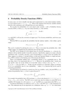
5 G(x)has been normalized so that the accumulated area under the curvebetween x + totals to unity. A cumulative distribution function, which totalsthe area under the normalized distribution curve is available and can be plotted as : Plot of Gaussian Function and Cumulative Distribution FunctionWhen the mean is set to zero ( = 0) and the standard deviation or variance is set to unity( = 1), we get the familiar normal distributionG(x) =1 2 e x2/2dx( )which is shown in the curve below. The normal distribution functionN(x)gives the prob-ability that a variate assumes a value in the interval [0,x]N(x) =1 2 x0e t2/2dt( ) : Plot of the Normalized Gaussian FunctionGaussian distributions have many convenient properties, so random variates with unknowndistributions are often assumed to be Gaussian, especially in physics, astronomy and variousaspects of engineering. Many common attributes such as test scores, height, etc.

6 , followroughly Gaussian distributions, with few members at the high and low ends and many inthe Algebra SystemsFunctionMapleMathematicaProbabili ty Density Functionstatevalf[pdf,dist](x) PDF[dist, x]- frequency of occurrence atxCumulative Distribution Functionstatevalf[cdf,dist](x) CDF[dist, x]- integral of probabilitydensity function up toxdist=normald[ , ]dist=NormalDistribution[ , ] = 0(mean) = 0(mean) = 1(std. dev.) = 1(std. dev.)Potential Averaging:7 Error FunctionThe Error function is obtained by integrating the normalized Gaussian x0e t2dt( )where the coefficient in front of the integral normalizeserf ( ) = 1. A plot oferfxoverthe range 3 x 3is shown as : Plot of the Error FunctionThe Error function is defined for all values ofxand is considered an odd function inxsinceerfx= erf ( x).The Error function can be conveniently expressed in terms of other Functions and series asfollows:erfx=1 (12,x2)( )=2x M(12,32, x2)=2x e x2M(1,32,x2)( )=2 n=0( 1)nx2n+1n!

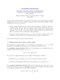
7 (2n+ 1)( )where ( )is the incomplete gamma function,M( )is the confluent hypergeometric functionof the first kind and the series solution is a Maclaurin Algebra SystemsFunctionMapleMathematicaError Functionerf(x) Erf[x] Complementary Error Functionerfc(x) Erfc[x]Inverse Error Functionfslove(erf(x)=s) InverseErf[s]Inverse Complementaryfslove(erfc(x)=s) InverseErfc[s] Error Functionwheresis a numerical value and we solve forxPotential :Transient conduction in a semi-infinite solid is governed by the diffusionequation, given as 2T x2=1 T twhere is thermal diffusivity. The solution to the diffusion equation is a function ofeither theerfxorerfcxdepending on the boundary condition used. For instance,for constant surface temperature, whereT(0,t) =TsT(x,t) TsTi Ts= erfc(x2 t)9complementary Error FunctionThe Complementary Error function is defined aserfcx= 1 erfx=2 xe t2dt( ) : Plot of the Complementary Error Functionand similar to the Error function, the Complementary Error function can be written in termsof the incomplete gamma Functions as follows:erfcx=1 (12,x2)( )As shown in Figure , the superposition of the Error function and the Complementary errorfunction when the argument is greater than zero produces a constant value of :In a similar manner to the transient conduction problem described for theerror function, the Complementary Error function is used in the solution of the diffusionequation when the boundary conditions are constant surface heat flux, whereqs=q0T(x,t) Ti=2q0( t/ )1/2kexp( x24 t) q0xkerfc(x2 t) x+Erfc xErf xErfc xFigure.

8 Superposition of the Error and Complementary Error Functionsand surface convection, where k T x x=0=h[T T(0,t)]T(x,t) TiT Ti= erfc(x2 t) [exp(hxk+h2 tk2)][erfc(x2 t+h tk)]11 Relations and Selected Values of Error Functionserf ( x) = erfxerfc ( x) = 2 erfcxerf 0 = 0erfc 0 = 1erf = 1erfc = 0erf ( ) = 1 0erfcx dx= 1/ 0erfc2x dx= (2 2)/ Ten decimal place values for selected values of the argument appear in Table Ten decimal place values 9999812 ApproximationsPower Series for Smallx(x <2)Sinceerfx=2 x0e t2dt=2 x0 n=0( 1)nt2nn!dt( )and the series is uniformly convergent, it may be integrated term by term. Thereforeerfx=2 n=0( 1)nx2n+1(2n+ 1)n!( )=2 {x1 0! x33 1!+x55 2! x77 3!+x99 4! }( )Asymptotic Expansion for Largex(x >2)Sinceerfcx=2 xe t2dt=2 x1te t2t dtwe can integrate by parts by lettingu=1tdv=e t2d dtdu= t 2dtv= 12e t2therefore x1te t2t dt=[uv] x xv du=[ 12te t2] x x12e t2t2dt13 Thuserfcx=2 {12xe x2 12 xe t2t2dt}( )Repeating the processntimes yields 2erfcx=12e x2(1x 12x3+1 322x5 + ( 1)n 11 3 (2n 3)2n 1x2n 1)++( 1)n1 3 (2n 1)2n xe t2t2ndt( )Finally we can write xex2erfcx= 1 + n=1( 1)n1 3 5 (2n 1)(2x2)n( )This series does not converge, since the ratio of thenthterm to the(n 1)thdoes not remainless than unity asnincreases.

9 However, if we takenterms of the series, the remainder,1 3 (2n 1)2n xe t2t2ndtis less than thenthterm because xe t2t2ndt < e x2< 0dtt2nWe can therefore stop at any term taking the sum of the terms up to this term as anapproximation of the function. The Error will be less in absolute value than the last termretained in the sum. Thus for largex,erfcxmay be computed numerically from theasymptotic expansion. xex2erfcx= 1 + n=1( 1)n1 3 5 (2n 1)(2x2)n= 1 12x2+1 3(2x2)2 1 3 5(2x2)3+ ( )14 Some other representations of the Error Functions are given below:erfx=2 e x2 n=0x2n+1(3/2)n( )=2x M(12,32, x2)( )=2x e x2M(1,32,x2)( )=1 (12,x2)( )erfcx=1 (12,x2)( )The symbols and represent the incomplete gamma Functions , andMdenotes the con-fluent hypergeometric function or Kummer s of the Error Functionddxerfx=2 e x2=ddx{2 x0e t2dt}( )Use of Leibnitz rule of differentiation of integrals gives:d2dx2erfcx=ddx2 e x2= 2 (2x)e x2( )d3dx3erfcx=ddx{ 2 (2x)e x2}=2 (4x2 2)e x2( )In general we can writedn+1dxn+1erfx= ( 1)n2 Hn(x)e x2(n= 0,1, )( )whereHn(x)are the Hermite Integrals of the Complementary Error Functioninerfcx= xin 1erfct dtn= 0,1,2.

10 ( )wherei 1erfcx=2 e x2( )i0erfcx= erfcx( )i1erfcx=ierfcx= xerfct dt=1 exp( x2) xerfcx( )i2erfcx= xierfct dt=14[(1 + 2x2) erfcx 2 xexp( x2)]=14[erfcx 2x ierfcx]( )The general recurrence formula is2ninerfcx=in 2erfcx 2xin 1erfcx(n= 1,2,3,..)( )Therefore the value atx= 0isinerfc 0 12n (1 +n2)(n= 1,0,1,2,3,..)( )It can be shown thaty=inerfcxis the solution of the differential equationd2ydx2+ 2xdydx 2ny= 0( )16 The general solution ofy + 2xy 2ny= 0 x ( )is of the formy=Ainerfcx+Binerfc ( x)( )Derivatives of Repeated Integrals of the Complementary ErrorFunctionddx[inerfcx] = ( 1)n 1erfcx(n= 0,1,2, )( )dndxn[ex2erfcx]= ( 1)n2nn!ex2inerfcx(n= 0,1,2, )( )17 Some Integrals Associated with the Error Function x20e t tdt= erfx( ) x0e t ydt= 2yerfx( ) 10e t2x21 +t2dt= 2ex2[1 {erfx}2]( ) 0e t x y+tdt= xexyerfc ( xy)x >0( ) 0e t2xt2+y2dt= 2yexy2erfc ( xy)x >0, y >0( ) 0e tx(t+y) tdt= yexyerfc (xy)x >0,y6= 0( ) 0e t xerf ( yt)dt= yx(x+y) 1/2(x+y)>0( ) 0e t xerf ( y/t dt=1xe 2 xyx >0,y >0( ) aerfc (t)dt= ierfc (a) + 2a= ierfc ( a)( ) a aerf (t)dt= 0( ) a aerfc(t)dt= 2a( ) aierfc (t)dt=i2erfc ( a) =12+a i2erfc (a)( ) ainerfc(t+cb)dt=bin+1erfc(a+cb)( )18 Numerical Computation of Error FunctionsThe power series form of the Error function is not recommended for numerical computationswhen the argument approaches and exceeds the valuex= 2because the large alternat-ing terms may cause cancellation, and because the general term is awkward to computerecursively.)