Probability Distributions - Duke University

1 Probability DistributionsCEE 201L. Uncertainty, Design, and OptimizationDepartment of Civil and Environmental EngineeringDuke UniversityPhilip Scott Harvey, Henri P. Gavin and Jeffrey T. ScruggsSpring 2022In the context of random variables, capital italics (X) represent an uncertain quantity (a randomvariable) and lower case italics (x) represent a particular value of that random variable. Randomvariables can bediscreteorcontinuous. Discreterandom variables can take on values that are members of a (finite or infinite) setof discrete values. IfXcan take on only positive whole numbers (the number of times ateam can win over all time), thenXis a discrete random variable with an infinitely largepopulation. IfXcan take on only whole numbers, between 0 and 23, (the hour of a day)thenXis a discrete random variable with a finite population.

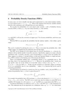
2 Continuousrandom variables can take on any value within finite or infinite bounds. Thepopulation of potential values of any continuous random variable is infinitely document focuses oncontinuousrandom Distributions of continuous random variablesThe properties of a random variable (rv)Xdistributed over the domain x X xare fullydescribed by itsprobability density functionor itscumulative distribution density function(PDF) ofXis the functionfX(x) such that for any twonumbersaandbwithin the domain x a b x,P[a < X b] = bafX(x)dxForfX(x) to be a proper distribution, it must satisfy the following two conditions: The PDFfX(x) is not negative;fX(x) 0 for all values ofxbetween xand x. The rule of total Probability holds; the total area underfX(x) is 1; x xfX(x)dx= distribution function(CDF) ofXis the functionFX(x) that gives, for anyspecified valuebbetween xand x, the Probability that the random variableXis less than or equalto the valuebis written asP[X b].

3 The CDF is defined byFX(x) =P[X x] = x fX(s)ds ,2 CEE 201L. Uncertainty, Design, and Optimization Duke University Spring 2022 , and a dummy variable of integration. So,P[a < X b] =FX(b) FX(a)By the first fundamental theorem of calculus, the functionsfX(x) andFX(x) are related asfX(x) =ddxFX(x)Some important characteristics of CDF s ofXare: CDF s,FX(x), are monotonic non-decreasing functions ofx. For any numbera,P[X > a] = 1 P[X a] = 1 FX(a) For any two numbersaandb, witha b,P[a < X b] =FX(b) FX(a) = bafX(x)dx(CC) BY-NC-NDApril 27, 2022 PSH, HPG, JTSP robability Distributions32 Statistics of random variablesTheexpectedormean valueof a continuous random variableXwith PDFfX(x) is thecentroidof the Probability density . X=E[X] = xfX(x)dxThe expected value of an arbitrary function ofX,g(X), with respect to the PDFfX(x) is g(X)=E[g(X)] = g(x)fX(x)dxThevarianceof a continuous random variableXwith PDFfX(x) and mean Xgives a quantitativemeasure of how much spread ordispersionthere is in the distribution ofxvalues.

4 The variance isthe expectation of (X X)2 2X V[X] =E[(X X)2]= (x X)2fX(x)dx= (x2 2 Xx+ 2X)fX(x)dx= x2fX(x)dx 2 X xfX(x)dx+ 2X fX(x)dx=E[X2] 2 XE[X] + but X=E[X] so ..=E[X2] the mean of the square minus the square of the meanThestandard deviation( ) ofXis X= V[X].Thecoefficient of variation( ) ofXis the standard deviation as a fraction of the mean:cX= X X .. for X6= 0 The is a normalized measure of dispersion and is a Probability density function,fX(x), is a value ofxsuch that the PDF is maximized;ddxfX(x) x=xmode= is a distribution with multiple ,xmed, is is the value ofxsuch thatP[X xmed] =P[X > xmed] =FX(xmed) = 1 FX(xmed) = (CC) BY-NC-NDApril 27, 2022 PSH, HPG, JTS4 CEE 201L. Uncertainty, Design, and Optimization Duke University Spring 2022 , and from a sample of values of a random variable (Sample Statistics)Consider afixed sampleofmspecific observed numerical values{x1, ,xm}drawn from apopu-lationwith CDFFX(x).

5 IfXis is a continuous random variable, it can take on any value withinpotentially infinite bounds. In such cases the population is infinitely large, and it is impossible toknow it s distributionFX(x) exactly. A random sample of the population can, however, be used toestimate the population statistics. A few sample statistics are: xmaxandxmin: the maximum and minimum values of the sample{x1, ,xm}xmin= mini(xi), i= 1, ,m xmax= maxi(xi), i= 1, ,m xavg: the arithmetic average of values of the sample{x1, ,xm}.. is the estimate of the population mean, X X xavg=1mm i=1xi xgm: the geometric average of values of the sample{x1, ,xm}xgm=[m i=1xi]1/m xhm: the harmonic average of values of the sample{x1, ,xm}xhm=[m i=11xi] 1 xmed: the median value of the sample, for which half of the sample is greater thanxmed. xmad: the average absolute deviation of the sample,xmad=1mm i=1|xi xavg| xsd: the standard deviation of values in the the sample.

6 Is the estimate of the population standard deviation, X X x2sd=1m 1m i=1(xi xavg)2 xcov: the coefficient of variation of the samplexcov= xsdxavg Sample statistics of a function of a sample{g(x1),g(x2), ,g(xm)}are analogously ..g(x)min= mini(g(xi)), i= 1, ,m g(x)max= maxi(g(xi)), i= 1, ,mg(x)avg=1mm i=1g(xi)g(x)2sd=1m 1m i=1(g(xi) g(x)avg)2 Importantly, note that in general,g(x)min6=g(xmin),g(x)avg6=g(xavg ), et cetera.(CC) BY-NC-NDApril 27, 2022 PSH, HPG, JTSP robability Distributions54 Empirical PDFs, CDFs, and exceedance ratesA PDF and a CDF of a sample of values can be computed directly from the sample. withoutassuming any particular Probability distributionA sample ofmrandom values can be sorted into increasing numerical order, so thatx1 x2 xi 1 xi xi+1 xN 1 the ordered sample there areidata points less than or equal toxi.

7 So, if the sample is represen-tative of the population, and the sample is big enough the Probability that a randomXis lessthan or equal to theithordered value isi/m. In other words,P[X xi] =i/m. Unless weknowthatno valueofXcan exceedxm, we must accept some Probability thatX > xm. So,P[X xm]should be less than 1. In such cases, the unbiased estimate1E[FX(xi)] forP[X xi] isi/(m+ 1)Theempirical CDFcomputed from a ordered sample ofmvalues is FX(xi) =im+ 1 Theempirical PDFis basically a histogram of the data. The followingMatlablines plot empiricalCDFs and PDFs from a vector of random data, =length(x);% number of values in the sample2x =sort(x);% sort the sample3x_avg =sum(x)/m;% average valueof the sample4x_med = x(round(m/2));% median valueof the sample5x_sd =sqrt(var(x));% standard deviationof ths sample6x_cov =abs(x_sd/x_avg);% c o e f f i c i e n t of variation of the sample7nBins =f l o o r(m/50);% number of bins in the histogram8[fx ,xx] =h i s t(x,nBins);% compute the histogram9fx = fx / m * nBins /(max(x)-min(x)));% scale the histogram to a PDF10F_x = ([1:m])/(m+1);% empirical CDF11subplot(121);bar(xx ,fx);% plo t empirical PDF12subplot(122);s t a i r s(sort(x), F_x).

8 % plo t empirical CDF13probability_X_gt_1 =sum(x>1) / (m+1)% fraction of the sample for which X> PDF f X(x) xavgxavg+ FX(x) xmedxavg = = = = [X>1] = number of values in the sample greater thanxiis (m i). If the sample is representative,the Probability of a value exceedingxiis Prob[X > xi] = 1 FX(xi) 1 i/(m+ 1). If themobservations were collected over a period of timeT, the averageexceedance rate(number of eventsgreater thanxiper unit time) is (xi) = (1 FX(xi))(m/T) (1 i/(m+ 1))(m/T). Gumbel,Statistics of extremes,Columbia Univ Press, 1958 Lasse Makkonen, Problems in the extreme value analysis, Structural Safety2008:30:405-419(CC) BY-NC-NDApril 27, 2022 PSH, HPG, JTS6 CEE 201L. Uncertainty, Design, and Optimization Duke University Spring 2022 , and common distributionsThe National Institute of Standards and Technology (NIST) lists properties of nineteen commonlyused Probability Distributions in their Engineering Statistics Handbook.

9 This section describes theproperties of seven Distributions . For each of these Distributions , this document provides figuresand equations for the PDF and CDF, equations for the mean and variance, the names ofMatlabfunctions to generate samples, and empirical Distributions of such Normal distributionThe Normal (or Gaussian) distribution is perhaps the most commonly used distribution notationX N( X, 2X) denotes thatXis a normal random variable with mean Xandvariance 2X. Thestandard normalrandom variable,Z, or z-statistic , is distributed asN(0,1).The Probability density function of a standard normal random variable is so widely used it has itsown special symbol, (z), (z) =1 2 exp( z22)Any normally distributed random variable can be defined in terms of the standard normal randomvariable, through the change of variablesX= X+ normally distributed, it has the PDFfX(x) = (x X X)=1 2 2 Xexp( (x X)22 2X)There is no closed-form equation for the CDF of a normal random variable.

10 Solving the integral (z) =1 2 z e u2/2duwould make you famous. Try it. The CDF of a normal random variable is expressed in terms of theerror function, erf(z). IfXis normally distributed,P[X x] can be found from the standardnormal CDFP[X x] =FX(x) = (x X X).Values for (z) are tabulated and can be computed, , theMatlabcommand ..Prob_X_le_x = normcdf(x,muX,sigX). The standard normal PDF is symmetric aboutz= 0,so ( z) = (z), ( z) = 1 (z), andP[X > x] = 1 FX(x) = 1 ((x X)/ X) = (( X x)/ X).The linear combination of two independent normal rv sX1andX2(with means 1and 2andvariances 21and 22) is also normally distributed,aX1 bX2 N(a 1 b 2,(a 1)2+ (b 2)2),and more specifically,aX b N(a X b ,(a X)2).(CC) BY-NC-NDApril 27, 2022 PSH, HPG, JTSP robability Distributions7 Given the Probability of a normal rv, , givenP[X x], the associated value ofxcan be foundfrom theinverse standard normalCDF,x X X=z= 1(P[X x]).