Transcription of Example experiment report for PHYS 342L - Purdue University
1 1 SS Dec 2001 Example experiment report for PHYS 342L The following report is written to help students in compiling their own reports for PHYS 342L class. Note that this report does not represent a real experiment and thus should be used only as an Example of style and form. The actual experiment reports will usually be longer as there is more material to cover. Disclaimer: The attached report has no scientific value, any resemblance of the theory, referred names or experiments presented in it with known theories, names or experiments is absolutely coincidental. It is expected, however, that students will describe real theory, use real names and present data from real experiment in their reports.
2 2 Measuring the magnitude of the gavitational field of Earth g. Boris Yolkin Department of Physics, Purdue University , , IN 47907 Abstract. In this work we determined the magnitude of Earth s gravitational field g by measuring free fall times for various objects released at different heights and using the Newton s 2nd law. We found that g= N/kg, which is in good agreement with the commonly accepted value of N/kg. 3 Introduction. The empirical fact that all material objects fall towards Earth if not supported has been known to humankind for as long as it has existed. Moreover, all live creatures on Earth consciously or unconsciously use this phenomenon in everyday life.
3 However, it has long been believed that heavier objects fall faster than lighter ones, and there was no exact theory to describe the motion of an object. Only in the 17th century, when Isaac Newton stated his famous motion laws and gave an exact relationship between force, mass, and acceleration, the quantitative description of motion became possible. In the following paper, we have used the laws of motion to measure the magnitude of the gravitational field of Earth. Theory. Newton s 2nd law states that any object would accelerate at a constant rate a if subjected to a constant force F [1]: a=F/m (1) where m, the proportionality coefficient, is called mass of an object.
4 The mass of an object should not be confused with its weight, as it is an intrinsic property of an object to resist acceleration (inertia), while weight refers to a force which attracts one object to Earth or some other usually larger object. While mass is constant1, weight may be different on different planets, or even in different places on the same planet. We can rewrite Eq. 1 in a more conventional form: F=ma (2) Surface of Earth F=mg h Fig. 1. Any object is a subject to force F=mg toward Earth 1 We consider only nonrelativistic case. 4 The force at which an object is attracted to Earth, or its weight, is also proportional to its mass (Fig.)
5 1) [2]: Fweight=mg (3) where g is proportionality coefficient. By comparing Eq. 2 and Eq. 3, one can see that g has the same units as a. Moreover, if an object is subjected to gravitational force we can combine Eqs. 2 and 3: ma=mg (4) or a=g (5) The last equation states that an object in free fall will accelerate toward earth with constant acceleration equal to g. The units of g are therefore m/s2, the same as for acceleration. Sometimes, however, units of N/kg are used to reflect the nature of g. defined by Eq. 3. Since acceleration is a second derivative of object s coordinate, we can rewrite Eq. 5 in the following form: gdthd=22 (6) where h is a height of an object from the surface of Earth.
6 Integrating Eq. 6 we get: gtgdtdtdht== 0 (7) ==tgtgtdth022 (8) 22thg= (9) The last equation shows that g can be easily determined if one measures free fall times t as a function of height h. In fact, a single pair of (h,t) is sufficient to uniquely determine the value of g. In this work, however, we will measure fall times for various heights to test the validity of Eq. 9 as well. Experimental apparatus and procedures In the first part of the experiment a kg solid aluminum ball was dropped down from different floors of a 10-story building and fall times were measured by a stop watch. The heights to different floors were measured by a conventional ruler. 5 T S B PE Computer Figure 2.
7 Experimental setup for measuring fall times as a function of height. T translation stage, S automated shutter, PE piezo-electric detector, B metal ball. In the second experiment fall times from heights up to 2 meters were measured by an automated setup (Fig. 2). Here, a container filled with small metal balls B and equipped with computer controlled shutter S is attached to a caret of a vertical translation stage T. Computer program slowly moves the caret T and releases metal balls at specified heights, one at a time. Simultaneously, the computer timer is started. The ball falls onto piezo-electric detector PE and that sends a stop signal to the computer timer.
8 The precision of the timer is 1 ms, and the height is determined to 5 mm. The experimental apparatus is described in more details in [3]. Data analysis, results and uncertainties. Part 1. The results of the first experiment are shown in Fig. 3. Here, the error in fall time measurement was estimated to be s and is mostly determined by the reaction time of the experimentalist. The height was measured by a ruler to 2 cm precision. Error bars for height are not shown in Fig. 3 since they are smaller than the size of the dots which represent the measured points. The general shape of this graph is well described with the quadratic dependence defined by Eq. 8, the solid line in Fig.
9 3 represents the expected dependence with the value g= m/s2. To analyze these data further, we used Eq. 9 to calculate the value of g for each data point, and the result of this calculation is shown in Fig. 4. , mTime, s Figure 3. Dependence of fall time on height. The solid line is theoretical simulation using Eq. 8 and g= m/s2. Error bars for measured values along X-axis are not shown as they are smaller than the size of the circles. 0510152036912151821242730 Height, mg, m/s/s Figure 4. The calculated value of g for different heights. The solid line corresponds to the average value m/s2. 7 The indicated error bars were calculated using the worst case scenario for each data point using the following equations: ()()22)(2)(2tthhgggtthhg + = += + (10) here g is the value calculated using equation (9), h= m and t= s are errors in measuring height and time, correspondingly, g+ and g- are error levels in positive and negative side of the calculated g value.
10 Based on these results, the average value of g can be calculated using least square fit as ( 2) m/s2. Corresponding straight line at g= m/s2 is also shown in Fig. 4. Part 2. In part II the computer measured 200 (h,t) points and the resulting dependence is shown in Fig. 5. The error level in these measurements is much smaller and is reflected in the visible noise in the curve. , mTime, s Fig. 5. Fall time versus height measured by computer controlled apparatus. 8 The data obtained by using automated data acquisition setup was analyzed in two ways. , mTime, , m2g, m/s Figure 6. Left: the data h(t) fitted using least square by Eq. (9), the best fit was obtained for g= m/s2.