Transcription of Excel 2019 Basic Quick Reference - Microsoft Office Training
1 Microsoft . Excel 2019 Basic Free Cheat Sheets Quick Reference Guide Visit The Excel 2019 Program Screen Keyboard Shortcuts General Quick Access Toolbar Title Bar formula Bar Close Button Open a workbook .. Ctrl + O. Create a new workbook .. Ctrl + N. File Tab Save a workbook .. Ctrl + S. Ribbon Print a workbook .. Ctrl + P. Close a workbook .. Ctrl + W. Name Help .. F1. Box Activate Tell Me field .. Alt + Q. Active Cell Spell check .. F7. Columns Calculate worksheets .. F9. Create absolute Reference .. F4. Scroll Bars Rows Navigation Move between cells .. , , , . Right one cell .. Tab Left one cell .. Shift + Tab Down one cell .. Enter Up one cell .. Shift + Enter Worksheet Tab Views Zoom Down one screen .. Page Down Slider To first cell of active row .. Home Enable End mode .. End Getting Started To cell A1 .. Ctrl + Home To last Ctrl + End Create a Workbook: Click the File Select an Entire Worksheet: Click the tab and select New or press Ctrl + Select All button where the Editing N.
2 Double-click a workbook. column and row headings meet. Cut .. Ctrl + X. Open a Workbook: Click the File tab Select Non-Adjacent Cells: Click the Ctrl + C. and select Open or press Ctrl + O. first cell or cell range, hold down the Paste .. Ctrl + V. Select a recent file or navigate to the Ctrl key, and select any non-adjacent location where the file is saved. cell or cell range. Undo .. Ctrl + Z. Redo .. Ctrl + Y. Preview and Print a Workbook: Click Cell Address: Cells are referenced by the coordinates made from their Find .. Ctrl + F. the File tab and select Print. column letter and row number, such Replace .. Ctrl + H. Undo: Click the Undo button on as cell A1, B2, etc. Edit active cell .. F2. the Quick Access Toolbar. Clear cell Delete Redo or Repeat: Click the Redo button on the Quick Access Toolbar. Formatting The button turns to Repeat once Jump to a Cell: Click in the Name everything has been re-done. Box, type the cell address you want Bold.
3 Ctrl + B. to go to, and press Enter. Italics .. Ctrl + I. Use Zoom: Click and drag the zoom Change Views: Click a View button in Underline .. Ctrl + U. slider to the left or right. the status bar. Or, click the View tab Open Format Cells Ctrl + Shift Select a Cell: Click a cell or use the and select a view. dialog box .. + F. keyboard arrow keys to select it. Select Ctrl + A. Recover an Unsaved Workbook: Select a Cell Range: Click and drag Restart Excel . If a workbook can be Select entire row .. Shift + Space to select a range of cells. Or, press recovered, it will appear in the Select entire column .. Ctrl + Space and hold down the Shift key while Document Recovery pane. Or, click Hide selected rows .. Ctrl + 9. using the arrow keys to move the the File tab, click Recover unsaved selection to the last cell of the range. workbooks to open the pane, and Hide selected Ctrl + 0. select a workbook from the pane. 2021 CustomGuide, Inc.
4 Click the topic links for free lessons! Contact Us: Edit a Workbook Basic Formatting Insert Objects Edit a Cell's Contents: Select a cell and click in Format Text: Use the commands in the Font Complete a Series Using AutoFill: Select the the formula Bar or double-click the cell. Edit group on the Home tab, or click the dialog box cells that define the pattern, a series of the cell's contents and press Enter. launcher in the Font group to open the dialog months or years. Click and drag the fill handle box. to adjacent blank cells to complete the series. Clear a Cell's Contents: Select the cell(s) and press the Delete key. Or, click the Clear Format Values: Use the commands in the button on the Home tab and select Clear Number group on the Home tab, or click the Contents. dialog box launcher in the Number group to Insert an Image: Click the Insert tab on the open the Format Cells dialog box. ribbon, click either the Pictures or Online Cut or Copy Data: Select cell(s) and click the Pictures button in the Illustrations group, Cut or Copy button on the Home tab.
5 Wrap Text in a Cell: Select the cell(s) that select the image you want to insert, and click contain text you want to wrap and click the Insert. Paste Data: Select the cell where you want to Wrap Text button on the Home tab. paste the data and click the Paste button in Insert a Shape: Click the Insert tab on the the Clipboard group on the Home tab. Merge Cells: Select the cells you want to ribbon, click the Shapes button in the merge. Click the Merge & Center button Illustrations group, and select the shape you Preview an Item Before Pasting: Place the list arrow on the Home tab and select a merge wish to insert. insertion point where you want to paste, click option. the Paste button list arrow in the Clipboard Hyperlink Text or Images: Select the text or group on the Home tab, and hold the mouse Cell Borders and Shading: Select the cell(s) graphic you want to use as a hyperlink. Click over a paste option to preview. you want to format.
6 Click the Borders the Insert tab, then click the Link button. button and/or the Fill Color button and Choose a type of hyperlink in the left pane of Paste Special: Select the destination cell(s), select an option to apply to the selected cell. the Insert Hyperlink dialog box. Fill in the click the Paste button list arrow in the necessary informational fields in the right pane, Clipboard group on the Home tab, and select Copy Formatting with the Format Painter: then click OK. Paste Special. Select an option and click OK. Select the cell(s) with the formatting you want to copy. Click the Format Painter button in Modify Object Properties and Alternative Text: Move or Copy Cells Using Drag and Drop: the Clipboard group on the Home tab. Then, Right-click an object. Select Edit Alt Text in Select the cell(s) you want to move or copy, select the cell(s) you want to apply the copied the menu and make the necessary position the pointer over any border of the formatting to.
7 Modifications under the Properties and Alt Text selected cell(s), then drag to the destination headings. cells. To copy, hold down the Ctrl key before Adjust Column Width or Row Height: Click and starting to drag. drag the right border of the column header or View and Manage Worksheets the bottom border of the row header. Double- Find and Replace Text: Click the Find & click the border to AutoFit the column or row Insert a New Worksheet: Click the Insert Select button, select Replace. Type the text according to its contents. Worksheet button next to the sheet tabs you want to find in the Find what box. Type the below the active sheet. Or, press Shift + F11. replacement text in the Replace with box. Click Basic Formulas the Replace All or Replace button. Delete a Worksheet: Right-click the sheet tab Enter a formula : Select the cell where you and select Delete from the menu. Check Spelling: Click the Review tab and click want to insert the formula .
8 Type = and enter the Spelling button. For each result, select the formula using values, cell references, Hide a Worksheet: Right-click the sheet tab a suggestion and click the Change/Change operators, and functions . Press Enter. and select Hide from the menu. All button. Or, click the Ignore/Ignore All button. Insert a Function: Select the cell where you Rename a Worksheet: Double-click the sheet want to enter the function and click the Insert tab, enter a new name for the worksheet, and Insert a Column or Row: Right-click to the right Function button next to the formula bar. press Enter. of the column or below the row you want to insert. Select Insert in the menu, or click the Reference a Cell in a formula : Type the cell Change a Worksheet's Tab Color: Right-click Insert button on the Home tab. Reference (for example, B5) in the formula or the sheet tab, select Tab Color, and choose click the cell you want to Reference . the color you want to apply.
9 Delete a Column or Row: Select the row or column heading(s) you want to remove. Right- SUM Function: Click the cell where you want to Move or Copy a Worksheet: Click and drag a click and select Delete from the contextual insert the total and click the Sum button in worksheet tab left or right to move it to a new menu, or click the Delete button in the Cells the Editing group on the Home tab. Enter the location. Hold down the Ctrl key while clicking group on the Home tab. cells you want to total, and press Enter. and dragging to copy the worksheet. Hide Rows or Columns: Select the rows or MIN and MAX functions : Click the cell where Switch Between Excel Windows: Click the columns you want to hide, click the Format you want to place a minimum or maximum View tab, click the Switch Windows button on the Home tab, select Hide & value for a given range. Click the Sum button, and select the window you want to Unhide, and select Hide Rows or Hide button list arrow on the Home tab and select make active.
10 Columns. either Min or Max. Enter the cell range you want to Reference , and press Enter. Freeze Panes: Activate the cell where you Basic Formatting want to freeze the window, click the View tab COUNT Function: Click the cell where you on the ribbon, click the Freeze Panes Change Cell Alignment: Select the cell(s) you want to place a count of the number of cells in button in the Window group, and select an want to align and click a vertical alignment a range that contain numbers. Click the Sum option from the list. , , button or a horizontal alignment button list arrow on the Home tab and select , , button in the Alignment group on the Count Numbers. Enter the cell range you Select a Print Area: Select the cell range you Home tab. want to Reference , and press Enter. want to print, click the Page Layout tab on the ribbon, click the Print Area button, and select Set Print Area. Adjust Page Margins, Orientation, Size, and Click the topic links for free lessons!