Finite Difference Method for Solving Differential Equations

1 Chapter Finite Difference Method for Ordinary Differential Equations After reading this chapter, you should be able to 1. Understand what the Finite Difference Method is and how to use it to solve problems. What is the Finite Difference Method ? The Finite Difference Method is used to solve ordinary Differential Equations that have conditions imposed on the boundary rather than at the initial point. These problems are called boundary-value problems. In this chapter, we solve second - order ordinary Differential Equations of the form bxayyxfdxyd =),',,(22, (1) with boundary conditions ayay=)( and byby=)( (2) Many academics refer to boundary value problems as position-dependent and initial value problems as time-dependent.

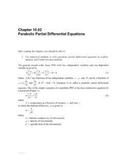
2 That is not necessarily the case as illustrated by the following examples. The Differential equation that governs the deflection y of a simply supported beam under uniformly distributed load (Figure 1) is given by EIxLqxdxyd2)(22 = (3) where =xlocation along the beam (in) =EYoung s modulus of elasticity of the beam (psi) =Isecond moment of area (in4) =quniform loading intensity (lb/in) =Llength of beam (in) The conditions imposed to solve the Differential equation are 0)0(==xy (4) 0)(==Lxy Clearly, these are boundary values and hence the problem is considered a boundary-value problem.

3 Chapter Figure 1 Simply supported beam with uniform distributed load. Now consider the case of a cantilevered beam with a uniformly distributed load (Figure 2). The Differential equation that governs the deflection y of the beam is given by EIxLqdxyd2)(222 = (5) where =xlocation along the beam (in) =EYoung s modulus of elasticity of the beam (psi) =Isecond moment of area (in4) =quniform loading intensity (lb/in) =Llength of beam (in) The conditions imposed to solve the Differential equation are 0)0(==xy (6) 0)0(==xdxdy Clearly, these are initial values and hence the problem needs to be considered as an initial value problem.

4 Figure 2 Cantilevered beam with a uniformly distributed load. q y L x q y L x Finite Difference Method Example 1 The deflection y in a simply supported beam with a uniform load qand a tensile axial load Tis given by EIxLqxEITydxyd2)(22 = ( ) where =xlocation along the beam (in) =Ttension applied (lbs) =EYoung s modulus of elasticity of the beam (psi) =Isecond moment of area (in4)

5 =quniform loading intensity (lb/in) =Llength of beam (in) Figure 3 Simply supported beam for Example 1. Given, 7200=Tlbs, 5400=qlbs/in, in 75=L, Msi 30=E, and 4in 120=I, a) Find the deflection of the beam at "50=x. Use a step size of "25= x and approximate the derivatives by central divided Difference approximation. b) Find the relative true error in the calculation of )50(y. Solution a) Substituting the given values, )120)(1030(2)75()5400()120)(1030(7200662 2 = xxydxyd )75( = ( ) Approximating the derivative 22dxyd at node i by the central divided Difference approximation, q y L x T T Chapter Figure 4 Illustration of Finite Difference nodes using central divided Difference Method .

6 21122)(2xyyydxydiii + + ( ) We can rewrite the equation as )75( )(276211iiiiiixxyxyyy = + + ( ) Since 25= x, we have 4 nodes as given in Figure 3 Figure 5 Finite Difference Method from 0=x to 75=x with 25= x. The location of the 4 nodes then is 00=x 2525001=+= +=xxx 50252512=+= +=xxx 75255023=+= +=xxx Writing the equation at each node, we get Node 1: From the simply supported boundary condition at 0=x, we obtain 01=y ( ) Node 2: rewriting equation ( ) for node 2 gives )75( )25(2227262123xxyyyy = + )2575)(25( =+ yyy =+ yyy ( ) Node 3: rewriting equation ( ) for node 3 gives )75( )25(2337362234xxyyyy = + )5075)(50( =+ yyy =+ yyy ( ) Node 4.

7 From the simply supported boundary condition at 75=x, we obtain 04=y ( ) 0=x 25=x 50=x 1=i 2=i 3=i 4=i 75=x 1 i i 1+i Finite Difference Method Equations ( ) are 4 simultaneous Equations with 4 unknowns and can be written in matrix form as = The above Equations have a coefficient matrix that is tridiagonal (we can use Thomas algorithm to solve the Equations ) and is also strictly diagonally dominant (convergence is guaranteed if we use iterative methods such as the Gauss-Siedel Method ).

8 Solving the Equations we get, = " )()50(22 = =yxyy The exact solution of the ordinary Differential equation is derived as follows. The homogeneous part of the solution is given by Solving the characteristic equation 010262= m =m Therefore, += The particular part of the solution is given by CBxAxyp++=2 Substituting the Differential equation ( ) gives )75( = )75( )(102)(726222xxCBxAxCBxAxdxd =++ ++ )75( )(1022726xxCBxAxA =++ )1022(102102xxCABxAx = + Equating terms gives = A = B 010226= CA Solving the above equation gives =B =C Chapter The particular solution then is + =xxyp The complete solution is then given by ++ + = Applying the following boundary conditions 0)0(==xy 0)

9 75(==xy we obtain the following system of Equations =+KK =+KK These Equations are represented in matrix form by = A number of different numerical methods may be utilized to solve this system of Equations such as the Gaussian elimination. Using any of these methods yields = Substituting these values back into the equation gives + =Unlike other examples in this chapter and in the book, the above expression for the deflection of the beam is displayed with a larger number of significant digits. This is done to minimize the round-off error because the above expression involves subtraction of large numbers that are close to each other.)

10 B) To calculate the relative true error, we must first calculate the value of the exact solution at 50=y. )50( )50( )50( )50(ey + = )50( e )50( =y The true error is given by tE = Exact Value Approximate Value ) ( =tE The relative true error is given by %100 Value TrueError True = t % = t %10 = t Finite Difference Method Example 2 Take the case of a pressure vessel that is being tested in the laboratory to check its ability to withstand pressure. For a thick pressure vessel of inner radius a and outer radius b, the Differential equation for the radial displacement u of a point along the thickness is given by 01222= +rudrdurdrud ( ) The inner radius 5 =a and the outer radius 8 =b, and the material of the pressure vessel is ASTM A36 steel.