Transcription of Forecasting Behavior with Age- Period-Cohort Models
1 Forecasting Behavior with Age- Period-Cohort ModelsHow APC Predicted the US Mortgage Crisis, but Also Does So Much More -2700 About the presenterDr. Breeden has been designing and deploying Forecasting systems since 1994. He co-founded Strategic Analytics in 1999, where he led the design of advanced analytic solutions including the invention of Dual-time Dynamics. He currently runs Prescient Models , which focuses on portfolio and account-level Forecasting solutions for lifetime value assessment, account management, and stress Breeden has created Models through the 1995 Mexican Peso Crisis, the 1997 Asian Economic Crisis, the 2001 Global Recession, the 2003 Hong Kong SARS Recession, and the 2007-2009 US Mortgage Crisis and Global Financial Crisis. These crises have provided Dr. Breeden with a rare perspective on crisis management and the analytics needs of executives for strategic decision-making. He has published over 40 academic articles and 6 patents.
2 The second edition of his book Reinventing Retail Lending Analytics: Forecasting , Stress Testing, Capital, and Scoring for a World of Crises was published by Riskbooksin Breeden received separate BS degrees in mathematics and physics in 1987 from Indiana University. He earned a in physics in 1991 from the University of Illinois studying real-world applications of chaos theory and genetic algorithms. Talk Outline What are Age- Period-Cohort Models ? What s the hidden story of the US Mortgage Crisis? Where else do APC Models apply? Are there implementation details we need to know?What are Age- Period-Cohort Models ?DefinitionsLexis Diagrams Between 1869 and 1875, Zuener, Brasche, Becker and Lexis invented a way to look at mortality rates by separating the data into year of birth ( cohort ) and year of death (period). Age is of course the age at death (period cohort ). In the 1960s and 70s, a rich literature developed in demography and epidemiology on how to estimate functions of age, period, and cohort using aggregate data like in the Lexis Period cohort (APC) Models Given an origination date (vintage), the age of the account is calendar date vintage date.
3 Functions of age , vintage , and time are then estimated. For binomially distributed events, this is The functions are most commonly estimated parametrically via splines or nonparametrically. Generalized Linear Model (GLM) estimation for splines, and Bayesian, Partial Least Squares, or Ridge Regression are used for the nonparametric (a,v,t)1-p(a,v,t) =F(a)+G(v)+H(t)F(a)G(v)H(t)a=t-vWhat s the hidden story of the US Mortgage Crisis?Use CaseJoint research with Jos Canals-Cerd , Federal Reserve Bank of Philadelphia, in log-odds of 60-89 DPD RateSuperprimePrimeSubprime-2-1012200020 0020022003200420052006200720082009 Relative change in log-oddsVintage DateSuperprimePrimeSubprimeF(a)G(v)H(t)E nvironment by stateCredit Quality by FICOL ifecycle by FICO logp(a,v,t)1-p(a,v,t) =F(a)+G(v)+H(t)Bayesian APC EstimationAdjusting for the Environment The environment function can reveal impacts for which no predictive factors are available.
4 The example below shows Hurricane Katrina s impact on mortgage delinquency. Later results are normalized any environmental impacts, like those shown in log-odds of 60-89 DPDDateCAFLLAMSTXLoan-level Modeling We use an APC decomposition initial step so that we capture all of the lifecycle and environment variation, and so that we control the linear trend ambiguity in age, vintage, time Models . (More on this later.) Then we keep the lifecycle and environment as fixed offsets in a GLM score using quarterly performance data. We include typical origination scoring factors and then test for the inclusion of vintage fixed effects (dummy variables) .logpi(a,v,t)1-pi(a,v,t) =offsetF(a)+H(t)()+c0+cjxijj=1ns +gvv=1nv gvScoring FactorsThe origination scoring factors and coefficients were typical for 1stlien, fixed rate excluded all of the exotic products, Option-ARMs. We re analyzing traditional mortgage 4: Output Coefficients from the GLM Analysis of Mortgage Delinquency.
5 Variables Coef. t-val Variables (cont.) Coef. t-val Intercept Source Channel Jumbo Loan source 1 0 Documentation source2 Full documentation 0 source7 Low documentation sourceT No documentation sourceU Documentation unknown Occupancy Fico at Origination Owner 0 up to 540 0 Non-owner 540 to 580 Other or Unknown 580 to 620 PMI 620 to 660 No 0 660 to 700 Yes 700 to 740 Unknown 740 to 780 Term 780 to 820 0 to 120 0 820+ 120 to 180 Loan to Value 180 to 240 0 to 0 240 to 360 to 360+ to Purpose to Purchase 0 to Refinance to 1 purposeU 1 to purposeZ DTI Note: The model specification includes also quarterly vintage dummies that are not explicitly reported in this table. APC Vintage Function versus Scoring Vintage Dummies The APC vintage function measures the net impact to log-odds of default for the variation in credit risk by vintage.
6 The scoring vintage dummies measure the vintage residual after scoring factors. By comparing, we see that only half of the vintage variation is explainable by scoring in log-odds of 60-89 DPDV intage DateAVT Vintage FunctionOrigination Score Vintage Fixed EffectsFRB SLOOS Survey Underwriting Standards The Federal Reserve publishes a Senior Loan Officer Opinion Survey (SLOOS). Self-reported changes in underwriting standards show a correlation of = to the vintage fixed effects, with the wrong in log-odds of 60-89 DPDL ooser standards Tighter standardsVintage DateNet Percentage of Domestic Respondents Tightening Standards for Mortgage Loans* AllNet Percentage of Domestic Respondents Tightening Standards for Mortgage Loans* PrimeScore Vintage Fixed EffectsFRB SLOOS Survey Consumer Loan Demand The same senior loan officers in the same survey report on consumer demand for loans. Consumer demand has a correlation of = the vintage effects.
7 When consumer demand is high, the loans are good consumer risk appetite is a real driver of credit in log-odds of 60-89 DPDLess Demand More DemandOrigination DateNet Percentage of Domestic Respondents Reporting Stronger Demand for Mortgage Loans* AllNet Percentage of Domestic Respondents Reporting Stronger Demand for Mortgage Loans* PrimeScore Vintage Fixed EffectsDrivers of Consumer Demand Historically, SLOOS-reported consumer mortgage demand is highly correlated to the 24-month change in mortgage interest rates. When offered interests fall over a sustained period, consumer demand in 30yr Mortgage Interest RateLess Demand More DemandOrigination DateSLOOS Mortgage Demand30yr Mortgage Intere Rate, 24m log-ratioWhere else do APC Models apply?ApplicationsOther Applications of APC Models Wine Forecasting SETI@home Dendrochronology eCommercecustomer lifetime value HR SalesFine Wine Value Forecasting Vincast million auction prices over a 10 year period Predicts wine price, starting with a Bayesian APC decomposition.
8 Wine is perfect for vintage Decomposition Chateau LafiteRothschildPrices actually drop through the first 5 years from LafiteBubble , caused by a flurry of interest from Chinese vintages are of the Wine Market The environment function (market index) for auctions prices has tracked Chinese wealth for the last @homeMember Analysis SETI@homeis the Search for Extraterrestrial Intelligence signal detection project. We analyzed 2 years of member data, analyzing activity rates, number of cpusapplied, and analysis return rates. Leading to member lifetime value estimates segmented by Country, OS, and software version. As an example of the lifetime value analysis, we show load, equivalent to usage for a website or spend on a credit Decompositionactivity(a,v,t)=activeaccou nts(a,v,t)activeaccounts(a=0,v,t) ChangeTenureActivity Ratio QualityVintage-50%0%50%100%Apr-99 Oct-99 May-00 Nov-00 Jun-01act-250%-200%-150%-100%-50%0%50%10 0%Apr-99 Oct-99 May-00 Nov-00 Jun-01ogenous Impact-350%-300%-250%-200%-150%-100%-50% 0%50%100%Apr-99 Oct-99 May-00 Nov-00 Jun-01 Exogenous ImpactDate-350%-300%-250%-200%-150%-100% -50%0%50%100%Apr-99 Oct-99 May-00 Nov-00 Jun-01 Exogenous ImpactDate-350%-300%-250%-200%-150%-100% -50%0%50%100%Apr-99 Oct-99 May-00 Nov-00 Jun-01 Exogenous ImpactDate-350%-300%-250%-200%-150%-100% -50%0%50%100%Apr-99 Oct-99 May-00 Nov-00 Jun-01 Exogenous ImpactDateEnvironmentRelative change in ChangeMonthMember Net Present Value Combining all factors, we predicted NPV for new members.
9 Allowing the SETI@homemanagers to target their development by OS and 2 Years40060080010001200s Returned in 2 Years10%4%0%020040060080010001200nSSnCLi nuxMac9therUnits Returned in 2 Years10%4%0%020040060080010001200 WinSSWinCLLinuxMac9 OtherUnits Returned in 2 Years10%4%0%020040060080010001200 WinSSWinCLLinuxMac9 OtherUnits Returned in 2 Years10%4%0%020040060080010001200 WinSSWinCLLinuxMac9 OtherUnits Returned in 2 Years10%4%0%180200100120140160180200ed in 2 Years10%20406080100120140160180200 Units Returned in 2 Years10%4%0%020406080100120140160180200 AustraliaBrazilCanadaFranceGermanyJapanM exicoew ZealandPolandRussian ..outh AfricaTaiwand Kingdomited StatesUnits Returned in 2 Years10%4%0%020406080100120140160180200 AustraliaBrazilCanadaFranceGermanyJapanM exicoNew ZealandPolandRussian ..South AfricaTaiwanUnited KingdomUnited StatesUnits Returned in 2 Years10%4%0%020406080100120140160180200 AustraliaBrazilCanadaFranceGermanyJapanM exicoNew ZealandPolandRussian.
10 South AfricaTaiwanUnited KingdomUnited StatesUnits Returned in 2 Years10%4%0%020406080100120140160180200 AustraliaBrazilCanadaFranceGermanyJapanM exicoNew ZealandPolandRussian ..South AfricaTaiwanUnited KingdomUnited StatesUnits Returned in 2 Years10%4%0%Dendrochronology Tree Ring Analysis Tree ring growth rates are driven by age of the tree, environmental conditions, and growth conditions for the individual of TreesAbiesconcolor(Gordon) Lindl. ex Hildebr302 Abieslasiocarpa(Hook.) Nutt3652 AbiesmagnificaA. Murray241 Castaneadentata(Marsh.) ex Engelm1562 PinusaristataEngelm256 PinusedulisEngelm2075 Pinusponderosa Douglas ex C. Lawson4998 Pseudotsugamenziesii(Mirb.) Franco Quercusalba L5324 Quercusalba L2690 Tsugacanadensis(L.) Carr1538 Tsugamertensiana(Bong.) Carriere1027 Tree Ring Decomposition Lifecycleslog(w)=F(a)+G(v)+H(t)Growth rate patterns differ by Ring Growth Lifecycle Phases Tree ring growth goes through different phases.