Transcription of Gaussian mixture models and the EM algorithm
1 Gaussian mixture models and the EM algorithmRamesh Sridharan These notes give a short introduction to Gaussian mixture models (GMMs) and theExpectation-Maximization (EM) algorithm , first for the specific case of GMMs, and thenmore generally. These notes assume you re familiar with basic probability and basic you re interested in the full derivation (Section 3), some familiarity with entropy and KLdivergence is useful but not strictly notation here is borrowed fromIntroduction to Probabilityby Bertsekas & Tsitsiklis:random variables are represented with capital letters, values they take are represented withlowercase letters,pXrepresents a probability distribution for random variableX, andpX(x)represents the probability of valuex(according topX).
2 We ll also use the shorthand notationXn1to represent the sequenceX1,X2,..,Xn, and similarlyxn1to representx1,x2,.., notes follow a development somewhat similar to the one inPattern Recognitionand Machine Learningby Review: the Gaussian distributionIf random variableXis Gaussian , it has the following PDF:pX(x) =1 2 e (x )2/2 2 The two parameters are , the mean, and 2, the variance ( is called the standard deviation).We ll use the terms Gaussian and normal interchangeably to refer to this save us some writing, we ll writepX(x) =N(x; , 2) to mean the same thing (where theNstands for normal). Parameter estimation for Gaussians: Suppose we have observationsXn1from a Gaussian distribution with unknown mean and known variance 2.
3 If we want to find the maximum likelihood estimate for the Contact: , we ll find the log-likelihood, differentiate, and set it to (xn1) =n i=1N(xi; , 2) =n i=11 2 e (x1 )2/2 2lnpXn1(xn1) =n i=1ln(1 2 ) 12 2(xi )2dd lnpXn1(xn1) =n i=11 2(xi )Setting this equal to 0, we see that the maximum likelihood estimate is =1N ixi: it s theaverage of our observed samples. Notice that this estimate doesn t depend on the variance 2! Even though we started off by saying it was known, its value didn t Gaussian mixture ModelsA Gaussian mixture model (GMM) is useful for modeling data that comes from one of severalgroups: the groups might be different from each other, but data points within the same groupcan be well-modeled by a Gaussian ExamplesFor example, suppose the price of a randomly chosen paperback book is normally distributedwith mean $ and standard deviation $ Similarly, the price of a randomly chosenhardback is normally distributed with mean $17 and variance $ Is the price of a ran-domly chosen book normally distributed?
4 The answer is no. Intuitively, we can see this by looking at the fundamental propertyof the normal distribution: it s highest near the center, and quickly drops off as you getfarther away. But, the distribution of a randomly chosen book is bimodal: the center ofthe distribution is near $13, but the probability of finding a book near that price is lowerthan the probability of finding a book for a few dollars more or a few dollars less. This isillustrated in Figure example: the height of a randomly chosen man is normally distributed with amean around 5 and standard deviation around . Similarly, the height of a randomlychosen woman is normally distributed with a mean around 5 and standard deviationaround 1Is the height of a randomly chosen person normally distributed?
5 The answer is again no. This one is a little more deceptive: because there s so muchoverlap between the height distributions for men and for women, the overall distribution isin fact highest at the center. But it s still not normally distributed: it s too wide and flat inthe center (we ll formalize this idea in just a moment). This is illustrated in Figure 1b. Theseare both examples ofmixtures of Gaussians: distributions where we have several groups and1In the metric system, the means are about 177 cm and 164 cm, and the standard deviations are about6 (dollars) (a) Probability density for paperback books (red),hardback books (blue), and all books (black, solid)556065707580 Height (inches) (b) Probability density for heights of women (red),heights of men (blue), and all heights (black, solid)Figure 1: Two Gaussian mixture models : the component densities (which are Gaussian ) areshown in dotted red and blue lines, while the overall density (which is not) is shown as asolid black data within each group is normally distributed.
6 Let s look at this a little more formallywith The modelFormally, suppose we have people numberedi= 1,..,n. We observe random variableYi Rfor each person s height, and assume there s an unobserved labelCi {M,F}foreach person representing that person s gender2. Here, the lettercstands for class . Ingeneral, we can have any number of possible labels or classes, but we ll limit ourselves to twofor this example. We ll also assume that the two groups have the same known variance 2,but different unknown means Mand F. The distribution for the class labels is Bernoulli:pCi(ci) =q1(ci=M)(1 q)1(ci=F)We ll also assumeqis known. To simplify notation later, we ll let M=qand F= 1 q,so we can writepCi(ci) = c {M,F} 1(ci=c)c(1)The conditional distributions within each class are Gaussian :pYi|Ci(yi|ci) = cN(yi; c, 2)1(ci=c)(2)2 Naive Bayes model, this is somewhat similar.
7 However, here our features are always Gaussian , and inthe general case of more than 1 dimension, we won t assume independence of the Parameter estimation: a first attemptSuppose we observe heightsY1=y1,..,Yn=yn, and we want to find maximumlikelihood estimates for the parameters Mand F. This is anunsupervised learningproblem:we don t get to observe the male/female labels for our data, but we want to learn parametersbased on those labels3 Exercise: Given the model setup in (1) and (2), compute the joint density of all the datapointspY1,..,YN(y1,..,yn) in terms of M, F, , andq. Take the log to find the log-likelihood, and then differentiate with respect to M. Why is this hard to optimize?Solution: We ll start with the density for a single data pointYi=yi:pYi(yi) = cipCi(ci)pYi|Ci(yi|ci)= ci( cN(yi; C, 2))1(ci=c)=qN(yi; M, 2) + (1 q)N(yi; F, 2)Now, the joint density of all the observations is:pYn1(yn1) =n i=1(qN(yi; M, 2) + (1 q)N(yi; F, 2)),and the log-likelihood of the parameters is thenlnpYn1(yn1) =n i=1ln( MN(yi; M, 2) + FN(yi; F, 2)),(3)We ve already run into a small snag: the sum prevents us from applying the log to the normaldensities inside.
8 So, we should already be a little worried that our optimization won t go assmoothly as it did for the simple mean estimation we did back in Section By symmetry,we only need to look at one of the means; the other will follow almost the same we dive into differentiating, we note thatdd N(x; , 2) =dd [1 2 e (x )22 2]=1 2 e (x )22 2 2(x )2 2=N(x; , 2) (x ) 2 Differentiating (3) with respect to M, we obtainn i=11 MN(yi; M, 2) + FN(yi; F, 2) MN(yi; M, 2)yi M 2= 0(4)At this point, we re stuck. We have a mix of ratios of exponentials and linear terms, andthere s no way we can solve this in closed form to get a clean maximum likelihood expression!3 Note that in a truly unsupervised setting, we wouldn t be able to tell which one of the two was maleand which was female: we d find two distinct clusters and have to label them based on their values after Using hidden variables and the EM AlgorithmTaking a step back, what would make this computation easier?
9 If we knew the hidden labelsCiexactly, then it would be easy to do ML estimates for the parameters: we d take all thepoints for whichCi=Mand use those to estimate Mlike we did in Section , and thenrepeat for the points whereCi=Fto estimate F. Motivated by this, let s try to computethe distribution forCigiven the observations. We ll start with Bayes rule:pCi|Yi(ci|yi) =pYi|Ci(yi|ci)pCi(ci)pYi(yi)= c {M,F}( cN(yi; c, 2))1(c=ci) MN(yi; M, 2) + FN(yi; F, 2)=qCi(ci)(5)Let s look at the posterior probability thatCi=M:pCi|Yi(M|yi) = MN(yi; M, 2) MN(yi; M, 2) + FN(yi; F, 2)=qCi(M)(6)This should look very familiar: it s one of the terms in (4)! And just like in that equation,we have to know all the parameters in order to compute this too. We can rewrite (4) interms ofqCi, and cheat a little by pretending it doesn t depend on M:n i=1qCi(M)yi M 2= 0(7) M=n i=1qCi(M)yin i=1qCi(M)(8)This looks much better: Mis a weighted average of the heights, where each height isweighted by how likely that person is to be male.
10 By symmetry, for F, we d compute theweighted average with weightsqCi(F).So now we have a circular setup: we could easily compute the posteriors overCn1if weknew the parameters, and we could easily estimate the parameters if we knew the posterioroverCn1. This naturally suggests the following strategy: we ll fix one and solve for the approach is generally known as theEM algorithm . Informally, here s how it works: First, we fix the parameters (in this case, the means Mand Fof the Gaussians) andsolve for the posterior distribution for the hidden variables (in this case,qCi, the classlabels). This is done using (6). Then, we fix the posterior distribution for the hidden variables (again, that sqCi, theclass labels), and optimize the parameters (the means Mand F) using the expectedvalues of the hidden variables (in this case, the probabilities fromqCi).