Transcription of Generalized Linear Models - UW Faculty Web Server
1 ' $. Generalized Linear Models Objectives: Systematic + Random. Exponential family. Maximum likelihood estimation & inference. & %. 45 Heagerty, Bio/Stat 571. ' $. Generalized Linear Models Models for independent observations Yi , i = 1, 2, .. , n. Components of a GLM: . Random component Yi f (Yi , i , ). f exponential family & %. 46 Heagerty, Bio/Stat 571. ' $.. Systematic component i = X i . i : Linear predictor Xi : (1 p) covariate vector : (p 1) regression coefficient . Link function E(Yi | X i ) = i g( i ) = X i . g( ) : link function & %. 47 Heagerty, Bio/Stat 571. ' $. Generalized Linear Models GLMs generalize the standard Linear model : Yi = X i + i.
2 Random: Normal distribution i N (0, 2 ).. Systematic: Linear combination of covariates i = X i .. Link: identity function i = i & %. 48 Heagerty, Bio/Stat 571. ' $. Generalized Linear Models GLMs extend usefully to overdispersed and correlated data: . GEE: marginal Models / semi-parametric estimation &. inference . GLMM: conditional Models / likelihood estimation & inference & %. 49 Heagerty, Bio/Stat 571. ' $. Exponential Family . y b( ). (?) f (y; , ) = exp + c(y, ). a( ). = canonical parameter = fixed (known) scale parameter Properties: If Y f (y; , ) in (?) then, E(Y ) = = b0 ( ). var(Y ) = b00 ( ) a( ).
3 & %. 50 Heagerty, Bio/Stat 571. ' $. Canonical link function: A function g( ) such that: = g( ) = (canonical parameter). Variance function: A function V ( ) such that: var(Y ) = V ( ) a( ). Usually : a( ) = w scale parameter w weight & %. 51 Heagerty, Bio/Stat 571. ' $. Examples of GLMS: logistic regression y = s/m where s=number of successes / m trials . m s f (y; , ) = (1 )m s s . y log( 1 ) + log(1 ) m = exp + log 1/m s = . = log( /(1 )). b( ) = log(1 ) = log[1 + exp( )]. 0 . = b ( ) = log[1 + exp( )].. = exp( )/[1 + exp( )] = . & %. 52 Heagerty, Bio/Stat 571. ' $. g( ) = log[ /(1 )] = . g : logit, log-odds function 1.
4 Var(y) = (1 ) . m V ( ) =. a( ) =. & %. 53 Heagerty, Bio/Stat 571. ' $. Poisson regression y = number of events (count). f (y; , ) = y exp( )/y! = exp [y log( ) log(y!)]. = . = log( ). b( ) = = exp( ). = b0 ( ) = exp( ) = . g( ) = = log( ). g : canonical link is log & %. 54 Heagerty, Bio/Stat 571. ' $. Poisson regression (continued). var(y) = . V ( ) =. a( ) =. Other examples: . gamma, inverse Gaussian (MN, Table ).. some survival Models (MN, Chpt. 13). & %. 55 Heagerty, Bio/Stat 571. ' $. Example: Seizure data (DHLZ ex. ). Clinical trial of progabide, evaluating impact on epileptic seizures.
5 Data: . age = patient age in years . base = 8-week baseline seizure count (pre-tx).. tx = 0 if assigned placebo; 1 if assigned progabide . Y1 , Y2 , Y3 , Y4 seizure counts in 4 two-week periods following treatment administration Models : . Linear model : Y4 = age + base + tx + .. Poisson GLM: log( 4 ) = age + base + tx & %. 56 Heagerty, Bio/Stat 571. ' $. Example: Seizure data (DHLZ ex. ). Linear regression Poisson regression est. Z est. Z. (Int) age base tx Q: should we use log(base) for Poisson regression? Q: why does inference regarding significance of TX differ? & %. 57 Heagerty, Bio/Stat 571.
6 60. 4.. 50.. 3.. log(y4 + ). 40.. 2. y4.. 30.. 1.. 20.. 10.. 0.. 0. 20 40 60 80 100 120 140 20 40 60 80 100 120 140. base base 10 12 14. 15. 10. 8. 6. 5. 4. 2. 0. 0. 0 20 40 60 0 20 40 60. y4[trt == 0] y4[trt == 1]. 58 Heagerty, Bio/Stat 571. Seizure Residuals vs. Fitted . 20. 10.. glmfit$resid lmfit$resid .. 0.. 10.. 0 10 20 30 40 10 20 30 40 50 60. lmfit$fitted glmfit$fitted 59 Heagerty, Bio/Stat 571. Seizure Residuals vs. Fitted, using predict(). 4.. 20.. 2. 10.. resid(glmfit). resid(lmfit).. 0.. 0.. 10.. 2.. 0 10 20 30 40 predict(lmfit) predict(glmfit). 60 Heagerty, Bio/Stat 571. ' $. Residual Diagnostics Used to assess model fit similarly as for Linear Models Q-Q plots for residuals (may be hard to interpret for discrete data ).
7 Residual plots: ? vs. fitted values ? vs. omitted covariates assessment of systematic departures assessment of variance function & %. 61 Heagerty, Bio/Stat 571. ' $. Residual Diagnostics Types of residuals for GLMs: 1. Pearson residual y bi r P. = pi V (b i ). X. (riP )2 = X2. 2. Deviance residual (see resid(fit)). p riD = sign(y . b) di X. (riD )2 = D(y, . b). 3. Working residual (see fit$resid). b i riW = (yi . bi ) = Zi bi . bi & %. 62 Heagerty, Bio/Stat 571. ' $. Fitting GLMS by Maximum Likelihood Solve score equations: . Uj ( ) = log L = 0 j = 1, 2, .. , p j log-likelihood: n . X . yi i b( i ).
8 Log L = + c(yi , ). i=1. ai ( ). X. = log Li = . log L X log Li i i i Uj ( ) = = . j i i i i j & %. 63 Heagerty, Bio/Stat 571. ' $. log Li 1 1. = (yi b0 ( i )) = (yi i ). i ai ( ) ai ( ). 1. i i = = 1/V ( i ). i i i = Xij j Therefore, Xn . i 1. Uj ( ) = Xij [ai ( ) V ( i )] (Yi i ). i=1. i & %. 64 Heagerty, Bio/Stat 571. ' $. GLM Information Matrix Either form: [In ](j, k) = cov[Uj ( ), Uk ( )]. 2.. log L. = E. j k Let's consider the second & %. 65 Heagerty, Bio/Stat 571. ' $. GLM Information Matrix .. [In ](j, k) = E Uj ( ). k " n #. X i 1. = E [ai ( ) V ( i )] (Yi i ).. i=1 k j Xn . i 1 i = [ai ( ) V ( i )].
9 I=1. j k justify & %. 66 Heagerty, Bio/Stat 571. ' $. Score and Information In vector/matrix form we have: . U1 ( ).. U2 ( ) .. U ( ) = .. Up ( ). i . i i i = 1 2 .. p . i = Xi i & %. 67 Heagerty, Bio/Stat 571. ' $. Score and Information n . X T. i 1. U ( ) = [ai ( ) V ( i )] (Yi i ). i=1.. and n . X T . i 1 i In = [ai ( ) V ( i )]. i=1.. & %. 68 Heagerty, Bio/Stat 571. ' $. Fisher Scoring Goal: Solve the score equations U ( ) = 0. Iterative estimation is required for most GLMs. The score equations can be solved using Newton-Raphson (uses observed derivative of score) or Fisher Scoring which uses the expected derivative of the score (ie.)
10 In ). & %. 69 Heagerty, Bio/Stat 571. ' $. Fisher Scoring Algorithm: (0). b Pick an initial value: . (j). b For j (j + 1) update via (j+1) (j). 1 (j). b b = + In b (j) b U ( ). b (j+1) . Evaluate convergence using changes in log L or k b (j) k. Iterate until convergence criterion is satisfied. & %. 70 Heagerty, Bio/Stat 571. ' $. Comments on Fisher Scoring: 1. IWLS is equivalent to Fisher Scoring (Biostat 570). 2. Observed and expected information are equivalent for canonical links. 3. Score equations are an example of an estimating function (more on that to come!). 4. Q: What assumptions make E[U ( )] = 0?