Transcription of Graphical and Tabular - The University of Texas at …
1 Graphical and TabularSummarization of DataOPRE 6301 Introduction and Re-cap..Descriptive statisticsinvolves arranging, summariz-ing, and presenting aset of datain such a way that usefulinformationis makes use of Graphical techniques and numerical de-scriptive measures (such as averages) to summarize andpresent the Graphical and Tabular methods presented here ap-ply to both entire populations and samples drawn ..Arandom variable, or simplyvariable, is a charac-teristic of a population or : Student grades, whichvariesfrom studentto student; and stock prices, whichvariesfrom stockto stock as well as over denoted by a capital letter:X,Y,Z..Thevaluesof a variable are possible observations or real-izations of that variable. The possible values of a variableusually land in a specified range. Examples:Student Grades: the interval [0,100].
2 Stock Prices: nonnegative real theobservedvalues of a variable. Examples:Grades of a sample of students:{34,78,64,90,76}Prices of stocks in a portfolio:{$ ,$ ,$ }2 Types of Data..Data fall into three main groups: Interval Data Nominal Data Ordinal DataDetails..3 Interval Data..Interval Dataare: real numbers, , heights, weights, prices, etc. also referred to operations can be performed on interval data,thus it is meaningful to talk about:2 * Height, orPrice + $1,and so Data..Nominal Dataare: namesorcategories, ,{Male, Female}and{single,Married, Divorced, Widowed}. also referred to operations donotmake sense for nominaldata ( , does Widowed / 2 = Married ?!).5 Ordinal Data..Ordinal Dataare also categorical in nature, but theirvalues have anorder. example :Course Ratings: Poor, Fair, Good, Very Good, Grades: F, D, C, B, Preferences: First Choice, Second Choice, , while it is still not meaningful to do arithmetic onordinal data ( , does 2 * fair = very good?)
3 !), we cansay things like:Excellent>Poor, orFair<Very GoodThat is, order is maintained no matter what numeric val-ues are assigned to each Hierarchy..Categorical?DataInterval DataNominal DataOrdinal DataNOrdered?YYNC ategorical Data7 example :For student grades, we haveCategorical?DataInterval { }Nominal {Pass | Fail}Ordinal {F, D, C, B, A}NOrdered?YYNC ategorical DataRank order to dataNO rank order to dataThus, information is lost as we move down this terms of calculations, we also have: All calculations are permitted onintervaldata. Only calculations involving a ranking process, or com-parison, are allowed forordinaldata. No calculations are allowed fornominaldata, otherthan counting the number of observations in each Data Tables and Graphs..Nominal (and ordinal) data can be summarized in a ta-ble that lists individual categories and their respectivefrequency counts, , afrequency can also use arelative frequency distribution,which lists the categories and theproportionwith whicheach :Student PlacementAreaFrequency Relative distributions and relative frequency distribu-tions can also be summarized asbar chartsandpiecharts, Data Tables and Graphs.
4 Interval data are typically summarized in for constructing a histogram is as 1: Partition the data range guidelines are: Use between 6 and 15 bins. One suggested formula(Sturges) is:Number of Classes = 1 + log(n)wherenis the total number of observations. All bins should have the same width. Use natural values for the bin width ( , 10 20,20 30, etc.).Step 2: Count the number of observations that fall ineach 3: Summarize the resulting frequency distributionas a table or as a bar :Monthly Long-Distance Telephone BillsWe have ( ): n= 200 (number of subscribers surveyed) Range = Largest Observation - Smallest Observation= $ $0= $ Suggested Number of Classes = 1 + log(n) = Since 120 = , Width = 15 seems to be a natural choice Number of Classes = 120/15 = 812 The results are:Lower Limit Upper Limit Frequency0157115303730451345609607510759 018901052810512014 Total20013 Observations.
5 About half (71+37=108)of the bills are small , less than $30 There are only a few telephonebills in the middle range.(18+28+14=60) 200 = 30% nearly a third of the phone billsare $90 or of Histograms..SymmetryA histogram is said to besymmetricif, when we drawavertical linedown the center of the histogram, the twosides are identical in shape and size:FrequencyVariableFrequencyVariableF requencyVariable15 SkewnessA skewed histogram is one with a long tail extending toeither the right or the left:FrequencyVariableFrequencyVariableP ositively SkewedNegatively Skewed16 ModalityAunimodalhistogram is one with asingle peak, whileabimodalhistogram is one withtwo peaks:FrequencyVariableUnimodalFrequency VariableBimodalA modal classis the class withthe largest number of observations17 Bell Shape (or Mound Shape)A special type ofsymmetric unimodalhistogram is onethat is bell shaped.
6 FrequencyVariableBell ShapedMany statistical techniques require that the population be bell the histogram helps verify the shape of the population in of Histograms..Comparing histograms often yields useful an example , contrast the following two histograms:The two courses have very different vs. bimodalspread of the marks (narrower | wider)19 Other Graphical Approaches..Stem and Leaf Display.. attempts to retain information about individual ob-servations that would normally be lost in the creation ofa : Split each observation into two parts, the observed value are several ways to split it up..We could split it at the decimal split it at the tens position (while rounding to thenearest integer in the ones position)241942 LeafStem241942 LeafStem20 Continue this process for all the observations in the long-distance-bills data.
7 Let each possible stem be a class and list all observed leafs for each stem, resulting in..Stem Leaf0 0000000000111112222223333345555556666666 7788889999991 0000011112333333344555556678899992 00001111123446667789993 00133558941244455895 335666 34587 0222245567898 3344578899999 0011222223334455599910 00134444669911 124557889 Thus, we still have access to our original data point s value!21 Histogram and stem-and-leaf display are similar..22 Ogive.. (pronounced Oh-jive ) is a graph of acumulativefrequency create an ogive in three steps..Step 1: Calculaterelative frequencies, defined asNumber of Observations in a ClassRelative Frequency = Total Number of ObservationsStep 2: Calculate thecumulativerelative frequenciesby adding the current class relative frequency to theprevious class cumulative relative frequency.
8 That is,we accumulate relative 3: Graph the cumulative relative the long-distance-bills data, we have..CumulativeLower Limit Upper Limit Relative Frequency Relative Frequency01571/200 =. =. =. =. =. =. =. =. = 1 What telephone bill value is at the 50th percentile?24 Two Nominal Variables..So far we havve looked at Tabular and Graphical tech-niques for one variable (either nominal or interval data).Acontingency table(also called a cross-classificationtable or cross-tabulation table) is used to describe therelationship betweentwonominal contingency table lists thefrequencyofeach combi-nationof the values of the two :Newspaper PreferenceA sample of newspaper readers was asked to report whichnewspaper they read: Globe and Mail (1), Post (2), Star(3), or Sun (4), and to indicate whether they were blue-collar worker (1), white-collar worker (2), or professional(3).
9 A contingency table is constructed as follows:This reader s response is captured as part of the total number on the contingency relative frequencies in columns 2 and 3 are similar,but there are large differences between columns 1 and 2and between columns 1 and tells us that blue collar workers tend to read dif-ferent newspapers from both white collar workers andprofessionals, and that white collar and professionals arequite similar in their newspaper the data from the contingency table, we can alsocreate a bar chart:Professionals tend to read the Globe & Mail more than twice as often as the Star or Interval Variables..Moving from nominal data to interval data, we are fre-quently interested in howtwointerval variables are explore this relationship, we employ ascatter dia-gram, which plots two variables against one variableis labeledXand is usuallyplaced on the horizontal axis, while the other,depen-dent variable,Y, is mapped to the vertical :Selling Price of a HouseA real estate agent wanted to know to what extent theselling price of a house is related to its size.
10 It appears that in fact there is a relationship: the greaterthe house size the greater the selling possible patterns are..Positive Linear RelationshipNegative Linear RelationshipWeak or Non-Linear RelationshipLinearity and Direction are two concepts we are ofteninterested Series Data..Observations measured at thesamepoint in time measured atsuccessivepoints in time example is the closing price of a stock for a particularday versus over a number of data graphed on aline chart, which plotsthe value of the variable on the vertical axis against thetime periods on the horizontal : Income TaxFrom 1987 to 1992, the tax was fairly flat. Starting 1993,there was a rapid increase in taxes until 2001. Finally,there was a downturn in ..Contingency Table, Bar ChartsScatter DiagramRelationship BetweenTwo VariablesFrequency and Relative Frequency Tables, Bar and Pie ChartsHistogram, Ogive, or Stem-and-Leaf DisplaySingle Set of DataNominalDataIntervalDataContingency Table, Bar ChartsScatter DiagramRelationship BetweenTwo VariablesFrequency and Relative Frequency Tables, Bar and Pie ChartsHistogram, Ogive, or Stem-and-Leaf DisplaySingle Set of DataNominalDataIntervalData34