Graphical Tools for Linear Structural Equation Modeling

1 Graphical Tools for Linear Structural Equation ModelingBryant Chen and Judea PearlUniversity of California, Los AngelesComputer Science DepartmentLos Angeles, CA, 90095-1596, USA(310) 825-3243 This paper surveys Graphical Tools developed in the past three decades that are applicable tolinear Structural Equation models (SEMs). These Tools permit researchers to answer key re-search questions by simple path-tracing rules, even for highly complex models. They includeparameter identification, causal effect identification, regressor selection, selecting instrumentalvariables, finding testable implications of a given model, identifying equivalent models andestimating counterfactual :causal effects, counterfactuals, equivalent models, goodness of fit, graphicalmodels, identification, Linear regression, misspecification testIntroductionStructural Equation Models (SEMs) are the dominant re-search paradigm in the quantitative, data-intensive behav-ioral sciences.

2 These models permit a researcher to expresstheoretical assumptions meaningfully, using equations , de-rive their consequences and test their statistical implicationsagainst data. The result is a powerful symbiosis betweentheory and data which underlies much of current researchin causal analysis, especially in therapy evaluation (Shroutet al., 2010), education testing and management (Muth n andMuth n, 2010), and personality research (Lee, 2012).While advances in Graphical models have had a transfor-mative impact on causal analysis and machine learning, onlya meager portion of these developments have found their wayto mainstream SEM literature which, by and large, prefersalgebraic over Graphical representations (Joreskog and Sor-bom, 1982; Bollen, 1989; Mulaik, 2009; Hoyle, 2012).

3 Oneof the reasons for this disparity rests on the fact that graph-ical techniques were developed for non-parametric analysis,while much of SEM research is conducted within the con-fines of Gaussian Linear models, to which matrix algebra andpowerful statistical tests are applicable. Among the tasksfacilitated by Graphical models are: model testing, identifi-cation, policy analysis, bias control, mediation, external va-lidity, and the analysis of counterfactuals and missing data(Pearl, 2014a).The purpose of this paper is to introduce psychometricresearchers to modern Tools of Graphical models and to de-scribe some of the benefits, as well as new insights thatgraphical models can provide. We will begin by introduc-ing basic definitions and Tools used in Graphical Modeling ,including graph construction, definitions of causal effects,and Wright s path tracing rules.

4 We then introduce more ad-vanced notions of graph separation, which were developedfor non-parametric analysis, but have simple and meaning-ful interpretation in Linear models. These Tools provide thebasis for model testing and identification criteria, discussedin subsequent sections. We then cover advanced applicationsof path diagrams including equivalent regressor sets, mini-mal regressor sets, and variance minimizing for causal ef-fect estimation. Lastly, we discuss counterfactuals and theircomputation in Linear SEMs before showing how the toolspresented in this paper provide simple solutions to five ex-amples representing non-trivial problems in SEM the exception of the Causal Effects among LatentVariables" section, we focus on models where all variablesare observable (often called path analysis models), allowingfor error terms to be correlated.

5 As Graphical techniqueswere originally developed for non-parametric models, theyhave not traditionally addressed the identification of effectsamong latent variables, which is impossible without para-metric assumptions. Instead, the presence of latent variableswas taken into account through the correlations they induceon the error terms. We will demonstrate how latent variablescan be summarized using error terms and briefly discuss howthe results in this paper, while not directly addressing causaleffects among latent variables, can nevertheless be applied totheir Diagrams and GraphsPath diagrams or graphs1are Graphical representations ofthe model structure. They were introduced by Sewell Wright(1921), who aimed to estimate causal influences from sta-tistical data on animal breeding.

6 Today, SEM is generally1We use both terms REPORT R-432 July 20152 BRYANT CHEN AND JUDEA PEARL implemented in software2, and, as a result, when users expe-rience unexpected behavior (due to unidentified parameters,for example) they are often at a loss as to the source of theproblem3. For the remainder of this section, we will reviewthe basics of path diagrams and provide users with simple,intuitive Tools that will be used to resolve questions of identi-fication, goodness of fit, and more using Graphical introduce path diagrams by way of example. Supposewe wish to estimate the effect of attending an elite collegeon future earnings. Clearly, simply regressing earnings oncollege rating will not give an unbiased estimate of the targeteffect. This is because elite colleges are highly selective, sostudents attending them are likely to have qualifications forhigh-earning jobs prior to attending the school.

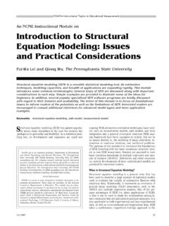
7 This back-ground knowledge can be expressed in the following SEMspecification. Throughout the paper, we will use lowercaseletters and the Greek letter to represent model Q1+U2Q2=c C+d Q1+U3S=b C+e Q2+U4,whereQ1represents the individual s qualifications prior tocollege,Q2represents qualifications after college,Ccontainsattributes representing the quality of the college attended,andSthe individual s 1a is a causal graph that represents this model spec-ification. Each variable in the model has a correspondingnode or vertex in the graph. Additionally, for each equa-tion, arrows are drawn from the independent variables to the(a)(b)Figure 1. (a) Model with latent variables (Q1andQ2) shownexplicitly (b) Same model with latent variables summarizeddependent variables.

8 These arrows reflect the direction ofcausation. In some cases, we may label the arrow with itscorresponding Structural coefficient as in Figure 1a. Errorterms are typically not displayed in the graph, unless theyare variablesQ1andQ2represent quantities that are notdirectly measurable. As a result, they arelatent this paper, we distinguish latent variables from observ-able variables in the graph by surrounding the former with adashed box. As we mentioned in the introduction , the pres-ence of latent variables is taken into account by the corre-lations they induce on the error terms4. For example, theeffect of the latent variables in Figures 1a is summarized byFigure 1b. We see that the effect of College on Salary inFigure 1a is now summarized by the coefficient in Figure1b.

9 Similarly, the bidirected arc betweenCandS(represent-ing the correlation of the error terms ofCandS) in Figure1b summarizes the correlation betweenCandSdue to thepathC Q1 Q2 S. The corresponding model is asfollows:Model C+USThe background information specified by Model 1 impliesthat the error term ofS,US, is not correlated withUC, andthis correlation is depicted in Figure 1a by the bidirected order to estimate , the causal effect of attending anelite college on future earnings, the coefficients must have aunique solution in terms of the covariance matrix or probabil-ity distribution over the observable variables,CandS. Thetask of finding this solution is known asidentificationand isdiscussed in a later section. In some cases, one or more co-efficients may not be identifiable, meaning that no matter thesize of the dataset, it is impossible to obtain point estimatesfor their values.

10 Indeed, we will see that the coefficients inModel 1 are not identified ifQ1andQ2are latent. However,if we include the strength of an individual s college appli-cation,A, as shown in Figure 2a, we obtain the followingmodel:2 Common software packages include AMOS (Arbuckle, 2005),EQS (Bentler, 1989), LISREL (J reskog and S rbom, 1989), andMPlus (Muth n and Muth n, 2010) among and Milan (2012) write, Identification is perhaps themost difficult concept for SEM researchers to understand. We haveseen SEM experts baffled and bewildered by issues of identifica-tion. 4 While we do not directly address the identification of causaleffects among latent variables, the results in this paper are neverthe-less applicable to this problem. See section Tools FOR Linear Structural Equation MODELING3(a)(b)Figure 2.