HIGHER-ORDER DIFFERENTIAL EQUATIONS

1 HIGHER-ORDER . DIFFERENTIAL EQUATIONS 3. Chapter Contents Theory of Linear EQUATIONS Initial-Value and Boundary-Value Problems homogeneous EQUATIONS Nonhomogeneous EQUATIONS Reduction of Order homogeneous Linear EQUATIONS with Constant Coefficients Undetermined Coefficients Variation of Parameters Cauchy Euler Equation Nonlinear EQUATIONS Linear Models: Initial-Value Problems Spring/Mass Systems: Free Undamped Motion Spring/Mass Systems: Free Damped Motion Spring/Mass Systems: Driven Motion Series Circuit Analogue Linear Models: Boundary-Value Problems Green's Functions Initial-Value Problems Boundary-Value Problems Nonlinear Models Solving Systems of Linear EQUATIONS Chapter 3 in Review We turn now to DEs of order two and higher. In the first six sections of this chapter we examine some of the underlying theory of linear DEs and meth- ods for solving certain kinds of linear EQUATIONS . The difficulties that surround HIGHER-ORDER nonlinear DEs and the few methods that yield analytic solutions of such EQUATIONS are examined next (Section ).

2 The chapter concludes with HIGHER-ORDER linear and nonlinear mathematical models (Sections , , and ) and the first of several methods to be considered on solving systems of linear DEs (Section ). Theory of Linear EQUATIONS 97. 97 9/22/09 5:55:51 PM. Theory of Linear EQUATIONS Introduction We turn now to DIFFERENTIAL EQUATIONS of order two or higher. In this section we will examine some of the underlying theory of linear DEs. Then in the five sections that follow we learn how to solve linear HIGHER-ORDER DIFFERENTIAL EQUATIONS . Initial-Value and Boundary-Value Problems Initial-Value Problem In Section we defined an initial-value problem for a general nth-order DIFFERENTIAL equation. For a linear DIFFERENTIAL equation, an nth-order initial-value problem is d ny d n 2 1y dy Solve: an 1x2 n 1 an 2 1 1x2 1 p 1 a1 1x2 1 a0 1x2y 5 g1x2. dx dx n 2 1 dx (1). Subject to: y1x02 y0, y 1x02 y1, p , y1n 2 12 1x02 yn 2 1. Recall that for a problem such as this, we seek a function defined on some interval I containing x0.

3 That satisfies the DIFFERENTIAL equation and the n initial conditions specified at x0: y(x0) y0, y (x0) . y1, .., y(n 1)(x0) yn 1. We have already seen that in the case of a second-order initial-value problem, a solution curve must pass through the point (x0, y0) and have slope y1 at this point. Existence and Uniqueness In Section we stated a theorem that gave conditions under which the existence and uniqueness of a solution of a first-order initial-value problem were guaranteed. The theorem that follows gives sufficient conditions for the existence of a unique solution of the problem in (1). Theorem Existence of a Unique Solution Let an(x), an 1(x), .. , a1(x), a0(x), and g(x) be continuous on an interval I, and let an(x) 0. for every x in this interval. If x x0 is any point in this interval, then a solution y(x) of the initial-value problem (1) exists on the interval and is unique. EXAMPLE 1 Unique Solution of an IVP. The initial-value problem 3y 5y y 7y 0, y(1) 0, y (1) 0, y (1) 0.

4 Possesses the trivial solution y 0. Since the third-order equation is linear with constant coefficients, it follows that all the conditions of Theorem are fulfilled. Hence y 0 is the only solution on any interval containing x 1. EXAMPLE 2 Unique Solution of an IVP. You should verify that the function y 3e2x e 2x 3x is a solution of the initial-value problem y 4y 12x, y(0) 4, y (0) 1. Now the DIFFERENTIAL equation is linear, the coef- ficients as well as g(x) 12x are continuous, and a2(x) 1 0 on any interval I containing x 0. We conclude from Theorem that the given function is the unique solution on I. The requirements in Theorem that ai(x), i 0, 1, 2, .., n be continuous and an(x) 0 for every x in I are both important. Specifically, if an(x) 0 for some x in the interval, then the solution of a linear initial-value problem may not be unique or even exist. For example, you should verify that the function y cx2 x 3 is a solution of the initial-value problem x2y 2xy 2y 6, y(0) 3, y (0) 1.

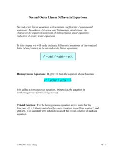
5 98 CHAPTER 3 HIGHER-ORDER DIFFERENTIAL EQUATIONS 98 9/22/09 5:55:52 PM. on the interval ( q, q) for any choice of the parameter c. In other words, there is no unique solution of the problem. Although most of the conditions of Theorem are satisfied, the obvious difficulties are that a2(x) x2 is zero at x 0 and that the initial conditions are also imposed at x 0. Boundary-Value Problem Another type of problem consists of solving a linear DIFFERENTIAL solutions of the DE. equation of order two or greater in which the dependent variable y or its derivatives are specified y at different points. A problem such as d 2y dy Solve: a2 1x2 1 a1 1x2 1 a0 1x2y 5 g1x2. dx2 dx (b, y1). Subject to: y1a2 y0, y1b2 y1. (a, y0). x is called a two-point boundary-value problem, or simply a boundary-value problem (BVP). I. The prescribed values y(a) y0 and y(b) y1 are called boundary conditions (BC). A solution of the foregoing problem is a function satisfying the DIFFERENTIAL equation on some interval I, con- FIGURE Colored curves are taining a and b, whose graph passes through the two points (a, y0) and (b, y1).

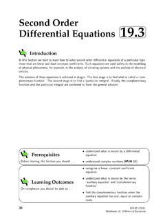
6 See FIGURE solutions of a BVP. For a second-order DIFFERENTIAL equation, other pairs of boundary conditions could be y (a) y0, y(b) y1. y(a) y0, y (b) y1. y (a) y0, y (b) y1, where y0 and y1 denote arbitrary constants. These three pairs of conditions are just special cases of the general boundary conditions A1 y(a) B1 y (a) C1. A2 y(b) B2 y (b) C2. The next example shows that even when the conditions of Theorem are fulfilled, a boundary-value problem may have several solutions (as suggested in Figure ), a unique solution, or no solution at all. EXAMPLE 3 A BVP Can Have Many, One, or No Solutions In Example 4 of Section we saw that the two-parameter family of solutions of the dif- ferential equation x 16x 0 is x c1 cos 4t c2 sin 4t. (2). x c2 = 1. (a) Suppose we now wish to determine that solution of the equation that further satisfies the c2 = 1. 1 2. boundary conditions x(0) 0, x(p/2) 0. Observe that the first condition 0 c1 cos 0 c2 = 1. 4. c2 sin 0 implies c1 0, so that x c2 sin 4t.

7 But when t p/2, 0 c2 sin 2p is c2 = 0. satisfied for any choice of c2 since sin 2p 0. Hence the boundary-value problem t x 1 16x 0, x 102 0, x1p>22 0 (3) (0, 0) ( /2, 0). c2 = 1. 1 2. has infinitely many solutions. FIGURE shows the graphs of some of the members of the one-parameter family x c2 sin 4t that pass through the two points (0, 0) and FIGURE The BVP in (3) of (p/2, 0). Example 3 has many solutions (b) If the boundary-value problem in (3) is changed to x 16x 0, x(0) 0, x 1p>82 0, (4). then x(0) 0 still requires c1 0 in the solution (2). But applying x(p/8) 0 to x c2. sin 4t demands that 0 c2 sin(p/2) c2 1. Hence x 0 is a solution of this new boundary-value problem. Indeed, it can be proved that x 0 is the only solution of (4). Theory of Linear EQUATIONS 99. 99 9/22/09 5:55:52 PM. (c) Finally, if we change the problem to x 16x 0, x(0) 0, x1p>22 1, (5). we find again that c1 0 from x(0) 0, but that applying x(p/2) 1 to x c2 sin 4t leads to the contradiction 1 c2 sin 2p c2 0 0.

8 Hence the boundary-value problem (5). has no solution. homogeneous EQUATIONS A linear nth-order DIFFERENTIAL equation of the form d ny d n 2 1y dy Note y 0 is always a an 1x2 1 a 1x2 1 p 1 a1 1x2 1 a0 1x2 y 0 (6). n n21 n21. solution of a homogeneous dx dx dx linear equation. is said to be homogeneous , whereas an equation d ny d n 2 1y dy an 1x2 n 1 an21 1x2 n21. 1 p 1 a1 1x2 1 a0 1x2 y g1x2 (7). dx dx dx with g(x) not identically zero, is said to be nonhomogeneous. For example, 2y 3y 5y 0. is a homogeneous linear second-order DIFFERENTIAL equation, whereas x2y 6y 10y ex is a nonhomogeneous linear third-order DIFFERENTIAL equation. The word homogeneous in this context does not refer to coefficients that are homogeneous functions as in Section ; rather, the word has exactly the same meaning as in Section We shall see that in order to solve a nonhomogeneous linear equation (7), we must first be able to solve the associated homogeneous equation (6). To avoid needless repetition throughout the remainder of this section, we shall, as a matter of course, make the following important assumptions when stating definitions and theorems about the linear EQUATIONS (6) and (7).

9 On some common interval I, Remember these assumptionss the coefficients ai(x), i 0, 1, 2, .., n, are continuous;. in the definitions and the right-hand member g(x) is continuous; and theorems of this chapter. an(x) 0 for every x in the interval. DIFFERENTIAL Operators In calculus, differentiation is often denoted by the capital letter D; that is, dy/dx Dy. The symbol D is called a DIFFERENTIAL operator because it transforms a differen- tiable function into another function. For example, D(cos 4x) 4 sin 4x, and D(5x3 6x 2) . 15x2 12x. HIGHER-ORDER derivatives can be expressed in terms of D in a natural manner: d dy d 2y d ny a b 5 2 5 D1Dy2 5 D2y and in general 5 D ny, dx dx dx dx n where y represents a sufficiently differentiable function. Polynomial expressions involving D, such as D 3, D2 3D 4, and 5x3D3 6x2 D2 4xD 9, are also DIFFERENTIAL operators. In general, we define an nth-order DIFFERENTIAL operator to be L an(x)Dn an 1(x)Dn 1 .. a1(x)D a0(x). (8). As a consequence of two basic properties of differentiation, D(cf (x)) c Df (x), c a constant, and D{ f (x) g(x)} Df (x) Dg(x), the DIFFERENTIAL operator L possesses a linearity property; that is, L operating on a linear combination of two differentiable functions is the same as the linear combination of L operating on the individual functions.

10 In symbols, this means L{af (x) bg(x)} aL( f (x)) bL(g(x)), (9). where a and b are constants. Because of (9) we say that the nth-order DIFFERENTIAL operator L is a linear operator. DIFFERENTIAL EQUATIONS Any linear DIFFERENTIAL equation can be expressed in terms of the D notation. For example, the DIFFERENTIAL equation y 5y 6y 5x 3 can be written as 100 CHAPTER 3 HIGHER-ORDER DIFFERENTIAL EQUATIONS 100 9/22/09 5:55:56 PM. D2y 5Dy 6y 5x 3 or (D2 5D 6)y 5x 3. Using (8), the nth-order linear dif- ferential EQUATIONS (6) and (7) can be written compactly as L( y) 0 and L( y) g(x), respectively. Superposition Principle In the next theorem we see that the sum, or superposition, of two or more solutions of a homogeneous linear DIFFERENTIAL equation is also a solution. Theorem Superposition Principle homogeneous EQUATIONS Let y1, y2, .. , yk be solutions of the homogeneous nth-order DIFFERENTIAL equation (6) on an interval I. Then the linear combination y c1 y1(x) c2 y2(x) .. ck yk(x), where the ci, i 1, 2.