INSTRUMENTATION AND CONTROL TUTORIAL 4 …

1 1 INSTRUMENTATION AND CONTROL TUTORIAL 4 SYSTEM RESPONSE This TUTORIAL is of interest to any student studying CONTROL systems and in particular the EC module D227 CONTROL System Engineering. On completion of this TUTORIAL , you should be able to do the following. Explain the output response of an ON/OFF CONTROL system. Explain and define the standard models for 1st and 2nd order systems. Explain and define the standard time dependant inputs to a system. Define a linear system and a linear time invariant system. Explain and calculate the response of a standard 1st order system to a step change in the input. Explain and calculate the response of a standard 1st order system to a ramp (velocity) change in the input.

2 Explain and calculate the response of a standard 1st order system to a sinusoidal change in the input. Explain how to find the overall gain of a system. Use partial fractions to solve responses. If you are not familiar with INSTRUMENTATION used in CONTROL engineering, you should complete the tutorials on INSTRUMENTATION Systems. In order to complete the theoretical part of this TUTORIAL , you must be familiar with basic mechanical and electrical science. You must also be familiar with the use of transfer functions and the Laplace Transform (see maths tutorials ). You must be able to convert polynomials into partial fractions.

3 2 1. INTRODUCTION A system may be defined as a set of connected things. We are concerned with engineering systems and we may define this more precisely as a set of connected elements designed to produce specified outputs when a given input is applied. System may include analogue elements or digital elements. First we will examine a special kind of simple system that uses ON/OFF CONTROL . 2. ON/OFF CONTROL Consider a system made up of a tank of liquid, a heater and a switch. When the switch is operated, power is supplied to the heater and the water gets hotter. The operation of the switch is the input action and the temperature of the water is the output action.

4 The output temperature is related to the power by the following formula. t mcTimeChange eTemperaturHeat x Specific x M assPOWER Figure 1 We may represent our system as a simple block. Figure 2 Often it is possible to represent the ratio of output/Input as a simple constant and give this constant the symbol G (it might be thought of as gain but this would not be strictly correct). In this example we have the following. mctP InputOutputG The system described is known as an OPEN LOOP SYSTEM because the signal path does not form a closed loop and there is no CONTROL over the temperature. When the switch is closed, the temperature will keep rising with time.

5 Now consider an improvement to the system by using a thermostatic controller and a thermocouple to measure the output. The desired temperature i (input) is set on the controller and the actual temperature o is the output of the system. The controller compares the measured temperature with the set temperature. If the water is too cold, the heater is turned on. If the temperature is too hot it is switched off. Suppose the temperature is low and correct and the set temperature is suddenly increased. This is called a step change. The thermostat will turn the heater on and the temperature will rise. Sometime later, the temperature reaches the correct value.

6 Figure 3 Ideally, the thermostat would switch off the heater at the precise moment that the correct temperature is reached. 3 In reality this cannot happen as heat will go on being put out after it is switched off and the thermostat has to detect that the temperature is too hot before it switches off. Consequently, the temperature rises above the correct value before being switched off and then the liquid starts to cool. It will cool to just below the correct value before the thermostat detects the error and switches the heater back on. The liquid is heated again and the process continues indefinitely producing a temperature time graph as shown. This graph is called the SYSTEM TIME RESPONSE GRAPH.

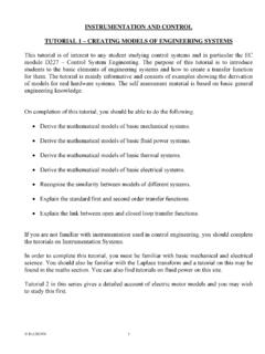
7 Figure 4 The block diagram of this system shows that the thermocouple turns the signal path into a closed loop so it is a CLOSED LOOP SYSTEM. Figure 5 The problem with all ON/OFF CONTROL is that the output must cycle between an OFF value and an ON value which are just above and below the SET value. If you bring the ON and OFF levels closer together the system must switch on and off more quickly. It is impossible to get precise CONTROL with this method. This is adequate for many systems such as central heating where the exact temperature is not important. Systems that need precision CONTROL (such as the movement of a machine tool) require a more sophisticated method of regulation and these are what we must study in detail.

8 3. RESPONSE OF CONTINUOUS CONTROL SYSTEMS We are going to discuss how to set about solving the way a given system behaves with respect to time. It should be noted, however, that time is not always the main variable but we will assume it is. We could, for example, be discussing how a robot manipulator moves in response to an input or how a valve on a pipe line moves in response to an input. STANDARD MODELS The first step is to derive a mathematical model along the lines shown in the previous tutorials . In those tutorials it was shown that the following models applied to several different systems that were analogues of each other. These are the standard first order and second order equations.

9 Standard 1st order equation. i = T d o/dt + o ..(1) Standard 2nd order equation. i = T2 d2 o/dt2 + 2 T d o/dt + o ..(2) T is a time constant and is a damping ratio. These will be discussed in greater detail later. T and are examples of system parameters or constants. 4 Before you can solve how the output changes with time, you have to decide how the input changes with time. For example, you might make a sudden change to the input or you might be changing it over a period of time. Let s look at this next. STANDARD INPUTS Standard inputs are usually listed in the following order. i. AN IMPULSE This is an instantaneous change in i lasting for zero length of time and returning to the initial value.

10 This is mostly applied to digital systems where instantaneous values are sampled by digital to analogue converters. It is also widely used as a standard input to a system to compare the responses of different systems. Figure 6 ii. A STEP CHANGE This is an instantaneous change in the input which then remains at the new value. i = H at all values of time after t= 0. H is the change or height of the step. Figure 7 iii. A RAMP OR VELOCITY CHANGE This is when the input changes at a constant rate. It is also called a velocity input. d i/dt = c or i = ct c is the rate of change (velocity). Figure 8 iv.