Transcription of Interpreting DSC Data - UC Santa Barbara
1 Interpreting DSC data TEMPO LABS, MATERIALS RESEARCH LABORATORY UCSB Written by Burton Sickler Interpreting DSC data 1 Table of Contents ANATOMY OF A PEAK .. 2 USING 2 IDENTIFYING TRANSITION EVENTS .. 2 SPLITTING A CURVE INTO SEGMENTS .. 3 SELECTING & HIDING SEGMENTS .. 3 SPLINING SEGMENTS .. 4 CHANGING TO A TEMPERATURE X-AXIS .. 5 IDENTIFYING THE EVENT ONSET 5 IDENTIFYING THE EVENT ENDSET TEMPERATURE .. 5 USING MANUAL SELECT .. 6 RECRYSTALLIZATION EVENTS .. 7 MELTING POINT PEAKS .. 8 MULTIPLE MELTING POINT PEAKS .. 8 POLYMORPHISM .. 9 OVERLAPPING PEAKS .. 9 RECRYSTALLIZATION POINT PEAKS.
2 10 MULTIPLE RECRYSTALLIZATION POINT 10 OTHER POSSIBLE PEAK EVENTS .. 11 GLASS TRANSITION POINTS (TG) .. 11 CURIE TRANSITION POINTS (TC) .. 11 Interpreting DSC data 2 Anatomy of a Peak A DSC event peak typically contains the following components: Baseline: This is the expected signal (or change in signal) if no transition event occurs ( if the enthalpy change of melting or Hfusion were zero). This is not always a flat line, as the specific heat capacity of a material is not guaranteed to be constant as temperature changes, or after a phase transition. First Tangent Line: This line is generated by an analytical program, (Proteus) and attempts to project a tangent along the most reasonable length of the phase transition s first peak.
3 The criteria for reasonable in this scenario would be the longest length of approximately consistent slope. Second Tangent Line: Similar to the first tangent line, this is a projection along the second length of the peak using similar methods. This is also generated by an analytical program. Onset: The onset of a transition event is where the tangent line intersects the baseline. Users may want to use the first tangent line to look at the onset of a melting transition or use the second tangent line to look at the onset of a recrystallization event. Endset: The endset of an event occurs at the intersection of the tangent line with the baseline on the second half of a peak.
4 Like the onset, users may choose the second tangent line to find the endset of a melting transition or the first tangent line to find the end point of a recrystallization event. Peak Apex: The location of the max peak value is subject to multiple variables. Its value is influenced by the thermal kinetics of the sample and the DSC system. The sample mass, shape, density, and crucible contact as well as the heating rate and gas environment will all impact at what temperature or time the phase transition will reach its maximum. As a result it is generally a poor indicator of a sample s properties.
5 Using Proteus Identifying Transition Events When a file is first opened in Proteus the default display use an x-axis of time and both temperature and signal along either y-axis. For the purposes of analyzing transition events users will find it useful to change the x-axis to temperature. This requires users will to first split the segments, hide isothermal portions and, if needed, spline segments together. Extrapolated Peak Second Tangent Line First Tangent Line Onset Endset Baseline Interpreting DSC data 3 Splitting a Curve into Segments To cut a measurement curve into segments users will need to left-click on their curve of interest, causing it to turn white.
6 Then, users will right click on the same curve to display a menu. From this menu select the Split Into Segments option. The curve should now be cut into multiple segments, of different colors, corresponding to each step in the programmed measurement. That is each segment corresponds to a dynamic or isothermal step according to the program used to gather the data . Selecting & Hiding Segments Once a curve is broken into its various steps each segment or set of segments may be selected or hidden. Right clicking on the background of the graph (the gray area) will open another menu allowing users to open the Segments window.
7 This window will show a list of the various segments that the curve has been cut into. Selecting or deselecting the check boxes next to each segment will allow users to hide or portion. Generally if users are interested in looking at transition events they can uncheck the initial heating periods and any isothermal segments that do not contain portions of the relevant peaks. For transition events with peaks that spill over into two segments, the segment will needed to be splined. Interpreting DSC data 4 Splining Segments In the Proteus analysis software, splining a set of segments will create a new line who s points include the data from the original segments.
8 This new line can then be treated as a dynamic step and manipulated accordingly. To spline your segments: Deselect any segments that you are not interested in so that they are hidden in the data display. Right click on any of the displayed segments to display a menu. Select Connect Segments Range (and spline) from the menu. A tool should appear at the top of the main display window, listing the segments you are about to connect. Continue connecting segments as needed. After deciding on each segment, the connected lines should now be present with the original components hidden.
9 The original line segments can always be restored by right clicking on the main background again and returning to the segments window. Interpreting DSC data 5 Changing to a Temperature X-Axis In the Proteus toolbar, at the top of the window, select the Temperature / time x-axis button. It should resemble a T / t with an arrow beneath it. The display will change the axis for you. After selecting this button, if isothermal segments are still present, then users will be given a warning. Continuing through this warning will automatically hide any isothermal segments.
10 Identifying the Event Onset Temperature First select the segment you are interested in analyzing by left clicking on the curve. Once selected thee curve should turn white. From the Proteus toolbar select the Onset icon. This will bring up two bounds on the main display as well as show the first derivative of your selected segment and add a second toolbar. The boundaries serve to identify which peak you want the software to analyze. Drag the first bound to the left of the peak, making sure to include a sizeable portion of your baseline signal. Place the second boundary at the apex or maximum value of the peak and then select Apply.