Transcription of John Schulman, Filip Wolski, Prafulla Dhariwal, Alec ...
1 Proximal Policy Optimization AlgorithmsJohn Schulman, Filip Wolski, Prafulla Dhariwal, Alec Radford, Oleg KlimovOpenAI{joschu, Filip , Prafulla , alec, propose a new family of policy gradient methods for reinforcement learning, which al-ternate between sampling data through interaction with the environment, and optimizing a surrogate objective function using stochastic gradient ascent. Whereas standard policy gra-dient methods perform one gradient update per data sample, we propose a novel objectivefunction that enables multiple epochs of minibatch updates. The new methods, which we callproximal policy optimization (PPO), have some of the benefits of trust region policy optimiza-tion (TRPO), but they are much simpler to implement, more general, and have better samplecomplexity (empirically). Our experiments test PPO on a collection of benchmark tasks, includ-ing simulated robotic locomotion and Atari game playing, and we show that PPO outperformsother online policy gradient methods, and overall strikes a favorable balance between samplecomplexity, simplicity, and IntroductionIn recent years, several different approaches have been proposed for reinforcement learning withneural network function approximators.}
2 The leading contenders are deepQ-learning [Mni+15], vanilla policy gradient methods [Mni+16], and trust region / natural policy gradient methods[Sch+15b]. However, there is room for improvement in developing a method that is scalable (tolarge models and parallel implementations), data efficient, and robust ( , successful on a varietyof problems without hyperparameter tuning).Q-learning (with function approximation) fails onmany simple problems1and is poorly understood, vanilla policy gradient methods have poor dataeffiency and robustness; and trust region policy optimization (TRPO) is relatively complicated,and is not compatible with architectures that include noise (such as dropout) or parameter sharing(between the policy and value function, or with auxiliary tasks).This paper seeks to improve the current state of affairs by introducing an algorithm that attainsthe data efficiency and reliable performance of TRPO, while using only first-order propose a novel objective with clipped probability ratios, which forms a pessimistic estimate( , lower bound) of the performance of the policy.
3 To optimize policies, we alternate betweensampling data from the policy and performing several epochs of optimization on the sampled experiments compare the performance of various different versions of the surrogate objec-tive, and find that the version with the clipped probability ratios performs best. We also comparePPO to several previous algorithms from the literature. On continuous control tasks, it performsbetter than the algorithms we compare against. On Atari, it performs significantly better (in termsof sample complexity) than A2C and similarly to ACER though it is much DQN works well on game environments like the Arcade Learning Environment [Bel+15] with discreteaction spaces, it has not been demonstrated to perform well on continuous control benchmarks such as those inOpenAI Gym [Bro+16] and described by Duan et al. [Dua+16].1 [ ] 28 Aug 20172 Background: Policy Policy Gradient MethodsPolicy gradient methods work by computing an estimator of the policy gradient and plugging itinto a stochastic gradient ascent algorithm.
4 The most commonly used gradient estimator has theform g= Et[ log (at|st) At](1)where is a stochastic policy and Atis an estimator of the advantage function at , the expectation Et[..] indicates the empirical average over a finite batch of samples, in analgorithm that alternates between sampling and optimization. Implementations that use automaticdifferentiation software work by constructing an objective function whose gradient is the policygradient estimator; the estimator gis obtained by differentiating the objectiveLPG( ) = Et[log (at|st) At].(2)While it is appealing to perform multiple steps of optimization on this lossLPGusing the sametrajectory, doing so is not well-justified, and empirically it often leads to destructively large policyupdates (see Section ; results are not shown but were similar or worse than the no clipping orpenalty setting). Trust Region MethodsIn TRPO [Sch+15b], an objective function (the surrogate objective) is maximized subject to aconstraint on the size of the policy update.
5 Specifically,maximize Et[ (at|st) old(at|st) At](3)subject to Et[KL[ old( |st), ( |st)]] .(4)Here, oldis the vector of policy parameters before the update. This problem can efficiently beapproximately solved using the conjugate gradient algorithm, after making a linear approximationto the objective and a quadratic approximation to the theory justifying TRPO actually suggests using a penalty instead of a constraint, ,solving the unconstrained optimization problemmaximize Et[ (at|st) old(at|st) At KL[ old( |st), ( |st)]](5)for some coefficient . This follows from the fact that a certain surrogate objective (which computesthe max KL over states instead of the mean) forms a lower bound ( , a pessimistic bound) on theperformance of the policy . TRPO uses a hard constraint rather than a penalty because it is hardto choose a single value of that performs well across different problems or even within a singleproblem, where the the characteristics change over the course of learning.
6 Hence, to achieve our goalof a first-order algorithm that emulates the monotonic improvement of TRPO, experiments showthat it is not sufficient to simply choose a fixed penalty coefficient and optimize the penalizedobjective Equation (5) with SGD; additional modifications are Clipped Surrogate ObjectiveLetrt( ) denote the probability ratiort( ) = (at|st) old(at|st), sor( old) = 1. TRPO maximizes a surrogate objectiveLCPI( ) = Et[ (at|st) old(at|st) At]= Et[rt( ) At].(6)The superscriptCPIrefers to conservative policy iteration [KL02], where this objective was pro-posed. Without a constraint, maximization ofLCPI would lead to an excessively large policyupdate; hence, we now consider how to modify the objective, to penalize changes to the policy thatmovert( ) away from main objective we propose is the following:LCLIP( ) = Et[min(rt( ) At,clip(rt( ),1 ,1 + ) At)](7)where epsilon is a hyperparameter, say, = The motivation for this objective is as follows.
7 Thefirst term inside the min isLCPI. The second term, clip(rt( ),1 ,1 + ) At, modifies the surrogateobjective by clipping the probability ratio, which removes the incentive for movingrtoutside of theinterval [1 ,1 + ]. Finally, we take the minimum of the clipped and unclipped objective, so thefinal objective is a lower bound ( , a pessimistic bound) on the unclipped objective. With thisscheme, we only ignore the change in probability ratio when it would make the objective improve,and we include it when it makes the objective worse. Note thatLCLIP( ) =LCPI( ) to first orderaround old( , wherer= 1), however, they become different as moves away from old. Figure 1plots a single term ( , a singlet) inLCLIP; note that the probability ratioris clipped at 1 or 1 + depending on whether the advantage is positive or + A >0rLCLIP011 A <0 Figure 1: Plots showing one term ( , a single timestep) of the surrogate functionLCLIPas a function ofthe probability ratior, for positive advantages (left) and negative advantages (right).
8 The red circle on eachplot shows the starting point for the optimization, ,r= 1. Note thatLCLIP sums many of these 2 provides another source of intuition about the surrogate objectiveLCLIP. It shows howseveral objectives vary as we interpolate along the policy update direction, obtained by proximalpolicy optimization (the algorithm we will introduce shortly) on a continuous control problem. Wecan see thatLCLIPis a lower bound onLCPI, with a penalty for having too large of a interpolation [KLt]LCPI=Et[rtAt]Et[clip(rt, 1, 1 +)At]LCLIP=Et[min(rtAt, clip(rt, 1, 1 +)At)]Figure 2: Surrogate objectives, as we interpolate between the initial policy parameter old, and the updatedpolicy parameter, which we compute after one iteration of PPO. The updated policy has a KL divergence ofabout from the initial policy, and this is the point at whichLCLIPis maximal. This plot correspondsto the first policy update on the Hopper-v1 problem, using hyperparameters provided in Section Adaptive KL Penalty CoefficientAnother approach, which can be used as an alternative to the clipped surrogate objective, or inaddition to it, is to use a penalty on KL divergence, and to adapt the penalty coefficient so that weachieve some target value of the KL divergencedtargeach policy update.
9 In our experiments, wefound that the KL penalty performed worse than the clipped surrogate objective, however, we veincluded it here because it s an important the simplest instantiation of this algorithm, we perform the following steps in each policyupdate: Using several epochs of minibatch SGD, optimize the KL-penalized objectiveLKLPEN( ) = Et[ (at|st) old(at|st) At KL[ old( |st), ( |st)]](8) Computed= Et[KL[ old( |st), ( |st)]] Ifd < , /2 Ifd > dtarg , 2 The updated is used for the next policy update. With this scheme, we occasionally see policyupdates where the KL divergence is significantly different fromdtarg, however, these are rare, and quickly adjusts. The parameters and 2 above are chosen heuristically, but the algorithm isnot very sensitive to them. The initial value of is a another hyperparameter but is not importantin practice because the algorithm quickly adjusts AlgorithmThe surrogate losses from the previous sections can be computed and differentiated with a minorchange to a typical policy gradient implementation.
10 For implementations that use automatic dif-ferentation, one simply constructs the lossLCLIPorLKLPEN instead ofLPG, and one performsmultiple steps of stochastic gradient ascent on this techniques for computing variance-reduced advantage-function estimators make use alearned state-value functionV(s); for example, generalized advantage estimation [Sch+15a], or the4finite-horizon estimators in [Mni+16]. If using a neural network architecture that shares parametersbetween the policy and value function, we must use a loss function that combines the policysurrogate and a value function error term. This objective can further be augmented by addingan entropy bonus to ensure sufficient exploration, as suggested in past work [Wil92; Mni+16].Combining these terms, we obtain the following objective, which is (approximately) maximizedeach iteration:LCLIP+V F+St( ) = Et[LCLIPt( ) c1LV Ft( ) +c2S[ ](st)],(9)wherec1,c2are coefficients, andSdenotes an entropy bonus, andLV Ftis a squared-error loss(V (st) Vtargt) style of policy gradient implementation, popularized in [Mni+16] and well-suited for usewith recurrent neural networks, runs the policy forTtimesteps (whereTis much less than theepisode length), and uses the collected samples for an update.
![arXiv:0706.3639v1 [cs.AI] 25 Jun 2007](/cache/preview/4/1/3/9/3/1/4/b/thumb-4139314b93ef86b7b4c2d05ebcc88e46.jpg)
![arXiv:1301.3781v3 [cs.CL] 7 Sep 2013](/cache/preview/4/d/5/0/4/3/4/0/thumb-4d504340120163c0bdf3f4678d8d217f.jpg)
![@google.com arXiv:1609.03499v2 [cs.SD] 19 Sep 2016](/cache/preview/c/3/4/9/4/6/9/b/thumb-c349469b499107d21e221f2ac908f8b2.jpg)