Transcription of Joint Displacements and Forces
1 1 Joint Displacements and Forces 1. Coordinate Systems y z x x z y Fig. 1: Coordinate System1 Fig. 2: Coordinate System2 (widely used and also applied in this course) (used in some formulations) 2. Sign Convention for Joint Displacements and Forces uy Fy y My ux Fx x Mx z Mz uz Fz Fig. 3: Sign convention for Displacements Fig.
2 4: Sign convention for Forces 3. Sign Convention for Two-dimensional Problems uy Fy z ux Mz Fx Fig. 5: Two-Dimensional Displacements Fig. 6: Two-Dimensional Forces 2 Stiffness Matrix for Truss Members in the Local Axes System Consider a truss member AB subjected to Forces (XA, YA) and (XB, YB) at joints A and B. YA YB XA XB A B Assume that the length of the member is L, its modulus of elasticity is E and cross-sectional area A.
3 The axial stiffness of the member, Sx = Load to produce unit deflection = EA/L Also assume that the member has no flexural or shear stiffness. If the Displacements of joints A and B are (uA, vA) and (uB, vB), the effect of the external Forces may result in the following cases. (uA=1) (vA=1) uA=1 vA=1 Sx uA Sx uA A B (uB=1) (vB=1) uB=1 vB=1 Sx uB Sx uB A B Equilibrium equations: Fx(A) = 0 XA = Sx uA + 0 Sx uB + 0.
4 (1) Fy(A) = 0 YA = 0 + 0 + 0 + 0 ..(2) Fx(B) = 0 XB = Sx uA + 0 + Sx uB + 0 ..(3) Fy(B) = 0 YB = 0 + 0 + 0 + 0 ..(4) Eqs. (1)~(4) can be summarized in matrix form as Sx 0 Sx 0 uA XA 0 0 0 0 vA YA Sx 0 Sx 0 uB XB 0 0 0 0 vB YB KmL umL = pmL ..(5) where KmL = The stiffness matrix of member AB in the local axis system, umL = The displacement vector of the member in the local axis system, and pmL = The force vector of the member in the local axis system = 3 Transformation of Stiffness Matrix from Local to Global Axes The member matrices formed in the local axes system can be transformed into the global axes system by considering the angles they make with the horizontal.
5 The local vectors and global vectors are related by the following equations. vBG vBL uBL B uBG vAG vAL A uAG uAL Local and global Joint Displacements of a truss member uAL = uAG cos + vAG sin ..(6) vAL = uAG sin + vAG cos ..(7) uBL = uBG cos + vBG sin ..(8) vBL = uBG sin + vBG cos ..(9) In matrix form uAL cos sin 0 0 uAG vAL sin cos 0 0 vAG uBL 0 0 cos sin uBG vBL 0 0 sin cos vBG umL = Tm umG.
6 (10) where Tm is called the transformation matrix for member AB, which connects the displacement vector umL in the local axes of AB with the displacement vector umG in the global axes. A similar expression can be obtained for the force vectors pmL and pmG; , pmL = Tm pmG ..(11) Eq. (5) can be rewritten as KmL Tm umG = Tm pmG ..(12) (Tm-1 KmL Tm) umG = pmG (TmT KmL Tm) umG = pmG ..(13) where TmT is the transpose of the transformation matrix Tm, which is also = Tm-1 If (TmT KmL Tm) is written as KmG, the member stiffness matrix in the global axis system, then C2 CS C2 CS CS S2 CS S2 [where C = cos , S = sin ] C2 CS C2 CS CS S2 CS S2 = = Sx KmG 4 Assembly of Stiffness Matrix and Load Vector of a Truss Assemble the global stiffness matrix and write the global load vector of the truss shown below.
7 Also write the boundary conditions [EA/L = Constant = 500 kip/ft]. 10k u8 D 20k u7 10 u2 u4 u6 u1 u3 u5 A B C 10 10 Member AB: (C = 1, S = 0) Member BC: (C = 1, S = 0) Member BD: (C = 0, S = 1) 1 2 3 4 3 4 5 6 3 4 7 8 1 0 1 0 1 1 0 1 0 3 0 0 0 0 3 KABG = 500 0 0 0 0 2 KBCG = 500 0 0 0 0 4 KBDG = 500 0 1 0 1 4 1 0 1 0 3 1 0 1 0 5 0 0 0 0 7 0 0 0 0 4 0 0 0 0 6 0 1 0 1 8 Member AD: (C = 1/2, S = 1/2) Member CD.
8 (C = 1/2, S = 1/2) 1 2 7 8 5 6 7 8 1 5 KADG = 500 2 KCDG = 500 6 7 7 8 8 1+ 0+ 1 0 XA 0+ 0+ 0 0 YA
9 1 0 1+1+0 0+0+0 1 0 0 0 XB 0 0 0+0+0 0+0+1 0 0 0 1 YB KG = 500 1 0 1+ pG = 0 0 0 0+ YC 0 0 0+ + 0+ 20 0 1 0+ 1+ + 10 Boundary Conditions: u1 = 0, u2 = 0, u3 = 0, u4 = 0, u6 = 0 1 2 3 4 5 6 7 8 1 2 3 4 5 6 7 8 5 Boundary Conditions, Support Reactions and Member Forces After assembly of the member stiffness matrices.
10 The equilibrium equations were 1 0 0 0 0 0 0 0 1 0 2 0 1 0 0 0 500 0 0 0 1 0 0 0 1 = 0 0 1 0 0 0 0 0 0 0 1 0 0 1 0 2 Applying the boundary conditions (u1 = 0, u2 = 0, u3 = 0, u4 = 0, u6 = 0), the equations are modified to u5 0 u5 = 10-3 ft 500 1 0 u7 = 20 u7 = 10-3 ft 0 2 u8 10 u8 = 10-3 ft Once Displacements are known, support reactions can be calculated from equilibrium equations.