L u(x,t) = (x,t)/ - Quarter Wave

1 Section : The Calculation Algorithm By Martin J. King, 07/05/02. copyright 2002 by Martin J. King. All Rights Reserved. Section : The Calculation Algorithm The Velocity and Pressure Equations for an Acoustic Element : In the previous section, the general equations for the displacement, the velocity, and the pressure were derived as functions of position and time. These relationships are restated below as Equations ( ), ( ), and ( ). Equations ( ), ( ), and ( ). ( ( I ) x ) ( ( + I ) x ) (I t ). ( x , t ) = ( C1 e + C2 e )e ( ( I ) x ) ( ( + I ) x ) (I t ). u( x , t ) = I ( C1 e + C2 e )e 2 ( ( I ) x ) ( ( + I ) x ) ( I t ).

2 P( x , t ) = I c ( C 1 ( I + ) e C 2 ( I + ) e )e If the two constants, C1 and C2, could be determined or eliminated from these equations, then the values of displacement, velocity, and pressure would be known everywhere within the transmission line. Having a background in mechanical engineering and experience performing structural finite element analyses, I decided to apply some of the methods used to derive one-dimensional truss elements to formulate a one-dimensional acoustic transmission line element. My one-dimensional acoustic transmission line element is shown in Figure along with a positive sign convention, the geometry definition, and the variables at end 1 and end 2.

3 Figure : One-Dimensional Acoustic Element L. p1 p2. u1 u2. S1 S2. u(x,t) = (x,t)/ t positive sign convention At end 1 : x = 0 (m) At end 2 : x = L (m). p1 pressure (Pa) p2 pressure (Pa). u1 velocity (m/sec) u2 velocity (m/sec). S1 area (m2) S2 area (m2). Page 1 of 11. Section : The Calculation Algorithm By Martin J. King, 07/05/02. copyright 2002 by Martin J. King. All Rights Reserved. Derivation of an Acoustic Element Transfer Matrix : Equations ( ) and ( ) for velocity and pressure contain two unknowns. If two values are assigned to any of the four variables (u1, u2, p1, or p2) from the acoustic element shown in Figure , then the remaining two variables can be used to eliminate the constants C1 and C2.

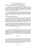
4 By careful selection of the two assigned values, convenient expressions for the two remaining variables result. In the following derivation the time (I t). varying term e has been dropped since it is common to every expression. Case 1 : u1 = 1 m/sec and u2 = 0 m/sec 2 (I L ) ( I L ). I c ( ( + I ) e + ( + I ) e ). p1 =. ( I L ) (I L ). (e e ). 2 ( L ). c e p2 = 2. (I L ) ( I L ). ( e +e ). Case 2 : u1 = 0 m/sec and u2 = 1 m/sec 2 ( L). c e p1 = 2. (I L ) ( I L ). ( e +e ). 2 ( I L ) (I L ). I c (( I ) e ( + I ) e ). p2 =. ( I L ) (I L ). (e e ). At this point, a demonstration problem would probably help the reader understand the pressure solutions for Cases 1 and 2.

5 Assume that the length L of the acoustic transmission line element is 1 meter and that the cross-sectional area is a constant m2. Since an expression for the fiber damping has not yet been derived, assume that the transmission line is empty. Also, define the excitation velocity as m/sec. For these assumptions, the resonances of the 1 m long closed end transmission line should be approximately : f = n x c / (2 x L) n = 1, 2, 3, and c = 342 m/sec f = 171 Hz for n = 1. = 342 Hz for n = 2. = 513 Hz for n = 3. Figures and show the pressure results for Cases 1 and 2 after applying these assumptions.

6 Page 2 of 11. Section : The Calculation Algorithm By Martin J. King, 07/05/02. copyright 2002 by Martin J. King. All Rights Reserved. Figure : Results for Case 1. Excitation at x = 0 : u(0) = 1, u(L) = 0. ( + j r) exp(j r L) + ( + j r) exp( j r L) . p 0 := j c . 2. r ( ( ) ( )). r d exp j r L exp j r L. 2 c r exp( L). 2. p L :=. r ( ( ). r d exp j r L exp j r L( )). 100. p0 10. r Pressure (Pa). 1000 Pa 1. pL. r 1000 Pa 1 .10. 3. 1 10 100. 1. r d Hz 100. 80. ( ). arg p 0. r 60. 40. Phase (deg). deg 20. ( ). 0. arg p L. r 20. deg 40. 60. 80. 100. 1 .10. 3. 1 10 100. 1. r d Hz Frequency (Hz). Acoustic Finite Element Model | Lumped Parameter Model |.

7 M | S0 L. p 0 = | Cab :=. 1 sec 2. | c 1 ( ). arg p 0 = |. | S0 . m sec m | p :=. p L = | j 1 Hz Cab 1 sec |. arg p L ( ) = 1. | p = arg ( p ) = Page 3 of 11. Section : The Calculation Algorithm By Martin J. King, 07/05/02. copyright 2002 by Martin J. King. All Rights Reserved. Figure : Results for Case 2. Excitation at x = L : u(0) = 0, u(L) = 1. ( j r) exp( j r L) ( + j r) exp(j r L) . p L := j c . 2. r ( ( ) ( )). r d exp j r L exp j r L. 2 c r exp( L). 2. p 0 :=. r ( ( ). r d exp j r L exp j r L ( )). 100. p0 10. r Pressure (Pa). 1000 Pa 1. pL. r 1000 Pa 1 .10. 3. 1 10 100. 1. r d Hz 100.

8 80. ( ). arg p 0. r 60. 40. Phase (deg). deg 20. ( ). 0. arg p L. r 20. deg 40. 60. 80. 100. 1 .10. 3. 1 10 100. 1. r d Hz Frequency (Hz). Acoustic Finite Element Model | Lumped Parameter Model |. m | S0 L. p 0 = | Cab :=. 1 sec 2. | c 1 ( ). arg p 0 = |. | S0 . m sec m | p :=. p L = | j 1 Hz Cab 1 sec |. arg p L ( ) = 1. | p = arg ( p ) = Page 4 of 11. Section : The Calculation Algorithm By Martin J. King, 07/05/02. copyright 2002 by Martin J. King. All Rights Reserved. A lot of information is contained in Figures and that warrants some further discussion and explanation. Lets start by looking closely at Figure , the same observations will apply to Figure unless otherwise noted.

9 The top plot is the pressure magnitude where it can be seen that sharp pressure peaks occur at the expected half wavelength frequencies. The pressure at both ends of the line spikes to extreme magnitudes at these frequencies. There are also some deep nulls in Figure but only in the pressure at the driven end. I would not classify these nulls as Quarter wavelength resonances even thought the frequencies are consistent with Quarter wavelength frequencies for the assumed length. At these frequencies, the length of the line is equivalent to a Quarter wavelength and a pressure distribution exists that tends to unload the driven end.

10 The pressure at the closed end is set by the velocity magnitude at the driven end and does not spike in a similar manner to the half wavelength modes. This is a velocity-controlled standing wave and therefore not what I would define as a true resonance. At the bottom of Figures and , the lumped parameter pressure is calculated and compared to the 1 Hz results from the acoustic transmission line element. This is really a check on the element static stiffness and it can be seen that both methods yield identical pressure magnitudes and phases. Also note the 180-degree difference in the phase calculated in Figure and Figure at the 1 Hz frequency.