Transcription of Lecture 3: Solving Equations Using Fixed Point Iterations
1 Cs412: introduction to numerical analysis09/14/10 Lecture 3: Solving Equations Using Fixed Point IterationsInstructor: Professor Amos Ron Scribes: Yunpeng Li, Mark Cowlishaw, Nathanael FillmoreOur problem, to recall, is Solving Equations in one variable. We are given a functionf, andwould like to find at least one solution to the equationf(x) = 0. Note that,a priori, we do notput any restrictions on the functionf; we do need to be able to evaluate the function: otherwise,we cannot even check that a given solutionx=ris true, , thatf(r) = 0. In reality, the mereability to be able to evaluate the function does not suffice. Weneed to assume some kind of goodbehavior.
2 The more we assume, the more potential we have, onthe one hand, to develop fastalgorithms for finding the root . At the same time, the more we assume, the fewer functions aregoing to satisfy our assumptions! This is a fundamental paradigm in Numerical from last week that we wanted to solve the equation:x3= sinxorx3 sinx= 0(1)We know that 0 is a trivial solution to the equation, but we would like to find a non-trivialnumeric solutionr. In a previous Lecture , we introduced an iterative process for finding roots ofquadratic Equations . We will now generalize this process into an algorithm for Solving equationsthat is based on the so-calledfixed Point Iterations , and therefore is referred to asfixed pointalgorithm.
3 In order to use Fixed Point Iterations , we need the followinginformation:1. We need to know that there is a solution to the We need to know approximately where the solution is ( an approximation to the solution).1 Fixed Point IterationsGiven an equation of one variable,f(x) = 0, we use Fixed Point Iterations as follows:1. Convert the equation to the formx=g(x).2. Start with an initial guessx0 r, whereris the actual solution ( root ) of the Iterate, usingxn+1:=g(xn) forn= 0,1,2, ..How well does this process work? We claim (xn) 0usingxn+1:=g(xn)as described in the process above. If(xn) 0convergesto a limitr, and the functiongis continuous atx=r, then the limitris a root off(x):f(r) = is this true?
4 Assume that (xn) 0converges to some valuer. Sincegis continuous, thedefinition of continuity implies thatlimn xn=r limn g(xn) =g(r)1 Using this fact, we can prove our claim:g(r) = limn g(xn) = limn xn+1= ,g(r) =r, and since the equationg(x) =xis equivalent to the original onef(x) = 0, weconclude thatf(r) = that, for proving this claim, we had to make some assumption ong(viz,gis a continuousfunction). This follows the general pattern: the more restrictions we put on a function, the betterwe can analyze the function real trick of Fixed Point Iterations is in Step 1, finding a transformation of the originalequationf(x) = 0 to the formx=g(x) so that (xn) 0converges.
5 Using our original example,x3= sinx, here are some sin 1(x3) 1x2+x+1+ x3 sinx3x2 cosx (x)Figure 1: Graphical Solution forx3= sinxWe can start withx0= 1, since this is a pretty good approximation to the root , as shown inFigure 1. To choose the best functiong(x), we need to determine how fast (and if)xnconverges toa solution. This is key, because different transformations of a singlef(x) = 0 tox=g(x) can resultin a sequence ofxnthat diverges, converges to the root slowly, or converges tothe root good way to measure the speed of convergence is to use the ratio of the errors betweensuccessive Iterations . The error at iterationncan be defined as:en:=xn r(2)2whereris the actual solution (an alternative definition, isen:=|xn r|.)
6 To measure the rate ofconvergence, we can take the ratio n+1between the error at iterationn+ 1 and the error at theprevious iteration: n+1:=en+1en=xn+1 rxn r(3)However, as you may have noticed, we are Using the actual solutionr, which we do not know,to calculate the errorenand the ratio n. For as long as we do not knowr, we can approximatethe erroren=xn r xn xn 1, and thus we can calculate the error ratio as: n+1=en+1en xn+1 xnxn xn 1(4)Note that the magnitude of the error ratio is what is important, so we can safely ignore Order of ConvergenceClearly, we would like the magnitude of the error ratio to be less than 1. We introduce now twonotions concerning orders of Linear ConvergenceLinear convergence requires that the error is reduced by at least a constant factor at each iteration:|en+1| c |en|(5)for some Fixed constantc <1.
7 We will study algorithms that converge much more quickly thanthis, in fact, we have already seen an algorithm (the square root algorithm) that quadratic ConvergenceQuadratic convergence requires that the error at each iteration is proportional to the square of theerror on the previous iteration:|en+1| c |en|2(6)for some constantc. Note that, in this case,cdoes not have to be less than 1 for the sequence toconverge. For example, if|en| 10 4, then|en+1|< c 10 8, so that a relatively large constant canbe offset by the Superlinear ConvergenceIn general, we can have|en+1| c |en| (7)for constantscand . If = 1, we have linear convergence, while if = 2 we have quadraticconvergence.
8 If >1 (but is not necessarily 2), we say we have superlinear is important to note that Equations 5, 6, and 7 providelower boundson the convergence is possible that an algorithm with quadratic convergencewill converge more quickly than thebound indicates in certain circumstances, but it will neverconverge more slowly than the boundindicates. Also note that these bounds are a better indicator of the performance of an algorithmwhen the errors are small (en 1). Experimental Comparison of Functions for Fixed Point IterationsWe Now return to our test the equationx3= sinx.(8)How do the functions we considered forg(x) compare? Table 1 shows the results of severaliterations Using initial valuex0= 1 and four different functions forg(x).
9 Herexnis the value ofxon thenth iteration and nis the error ratio of thenth iteration, as defined in Equation (x) =3 sinxg(x) =sinxx2g(x) =x+ sinx x3g(x) =x sinx x3cosx 3x2x1 1 2 3 4 26 27 1: Comparison of Functions for Fixed Point IterationsWe can see from the table that when we chooseg(x) =3 sinxorg(x) =x sinx x3cos(x) 3x2(columns1 and 4, respectively), the algorithm does converge to with the error ratio nfar less than 1. However, when we chooseg(x) =sinxx2, the error ratio is greater than 1 and theiteration do not converge. Forg(x) =x+ sinx x3, the error ratio is very close to 1. It appearsthat the algorithm does converge to the correct value, but very is there such a disparity in the rate of convergence?
10 2 Error Analysis of Fixed Point IterationsIn order to carry our analysis of Fixed Point Iterations , we assume thatgis differentiable. Note thecontinued theme: the more we restrict a function, the betterour tools are for analyzing the function4numerically. We previously assumedgto be continuous; now we raised the bar and assume it tobe would like to see howgis behaving in the area around the solution,r. For this, we will usethe Taylor expansion with remainder. Remember that, for anydifferentiable functiong, and forany two valuesx, a, there existscsuch thatg(x) =g(a) +g (c) (x a).(9)We don t know what the precise value ofcis, but we know that it exists and is Testing for DivergenceSubstitutingxnforxandr(the analytic solution) fora, we can use Equation 9 to provide a testfor divergence:en+1=xn+1 r=g(xn) g(r)= (xn r) g (cn)cnbetweenxnandr=en g (cn)(10)Asxnapproachesr,cn(which is betweenxnandr) is getting closer tor, and, thereforeg (cn) g (r).