Transcription of Lecture 4: Convolution - MIT OpenCourseWare
1 4 ConvolutionIn Lecture 3 we introduced and defined a variety of system properties towhich we will make frequent reference throughout the course. Of particularimportance are the properties of linearity and time invariance, both becausesystems with these properties represent a very broad and useful class and be-cause with just these two properties it is possible to develop some extremelypowerful tools for system analysis and linear system has the property that the response to a linear combina-tion of inputs is the same linear combination of the individual responses. Theproperty of time invariance states that, in effect, the system is not sensitive tothe time origin.
2 More specifically, if the input is shifted in time by someamount, then the output is simply shifted by the same importance of linearity derives from the basic notion that for a linearsystem if the system inputs can be decomposed as a linear combination ofsome basic inputs and the system response is known for each of the basic in-puts, then the response can be constructed as the same linear combination ofthe responses to each of the basic inputs. Signals (or functions) can be decom-posed as a linear combination of basic signals in a wide variety of ways. Forexample, we might consider a Taylor series expansion that expresses a func-tion in polynomial form.
3 However, in the context of our treatment of signalsand systems, it is particularly important to choose the basic signals in the ex-pansion so that in some sense the response is easy to compute. For systemsthat are both linear and time -invariant, there are two particularly usefulchoices for these basic signals: delayed impulses and complex this Lecture we develop in detail the representation of both continuous- time and discrete - time signals as a linear combination of delayed impulsesand the consequences for representing linear, time -invariant systems. The re-sulting representation is referred to as Convolution . Later in this series of lec-tures we develop in detail the decomposition of signals as linear combina-tions of complex exponentials (referred to as Fourier analysis) and theconsequence of that representation for linear, time -invariant developing Convolution in this Lecture we begin with the representa-tion of discrete - time signals and linear combinations of delayed impulses.
4 Aswe discuss, since arbitrary sequences can be expressed as linear combina-tions of delayed impulses, the output for linear, time -invariant systems can beSignals and Systems4-2expressed as the same linear combination of the system response to a delayedimpulse. Specifically, because of time invariance, once the response to oneimpulse at any time position is known, then the response to an impulse at anyother arbitrary time position is also developing Convolution for continuous time , the procedure is muchthe same as in discrete time although in the continuous- time case the signal isrepresented first as a linear combination of narrow rectangles (basically astaircase approximation to the time function).
5 As the width of these rectan-gles becomes infinitesimally small, they behave like impulses. The superposi-tion of these rectangles to form the original time function in its limiting formbecomes an integral, and the representation of the output of a linear, time -in-variant system as a linear combination of delayed impulse responses also be-comes an integral. The resulting integral is referred to as the Convolution in-tegral and is similar in its properties to the Convolution sum for discrete -timesignals and systems. A number of the important properties of Convolution thathave interpretations and consequences for linear, time -invariant systems aredeveloped in Lecture 5.
6 In the current Lecture , we focus on some examples ofthe evaluation of the Convolution sum and the Convolution ReadingSection , Introduction, pages 69-70 Section , The Representation of Signals in Terms of Impulses, pages 70-75 Section , discrete - time LTI Systems: The Convolution Sum, pages 75-84 Section , Continuous- time LTI Systems: The Convolution Integral, pages88 to mid-90c-7T:X1 ITkiv%\ r -L ,tY%3-InAvr-causal'4s~wSTM rEcY:% clecorpose pt 5 pwLinvo GL Lineer comet' C 0'sM baSic V Sina-tha. respolase eqs toLT I SWs ens-e g Convo + Co,x[-I] x[0] 1 x[2]-l IOJ fr 2x[0]x[O]8a[n] n-1 0 I2X[1] x[1]8[n-1]-1 0 I 2x[-I]8[n+1]0-0 --*- n-1 0 I 2X[-] x [-2]8[n +2]0--0-0 n-1 0 1 2x[o]8[n]+x(I] 8[n -1]+ x [-I]8[n+ ]+.)
7 --+X kr=2 x[k]8[n-k]k= general discrete - time signal expressedas a superposition ofweighted, delayed vA6.~iIrkv"O' "TVNVQI;Q,, ,Signals and Convolution sumfor linear, time -invariant discrete -timesystems expressingthe system output as aweighted sum ofdelayed unit )x[ x[2]-1 0 I 2X 10{ x[0]8[n]n-I 0 1 2X x[1]8[n+1]x[2] x[-2]8[n+2]91T n-1 0 i 2-0-0-0-0-- m- x [0] h [n]0000x [ 1] h [n-I]x [-I] h [n+ [-2] h [ ] interpretation ofthe Convolution sumfor an LTI individualsequence value can beviewed as triggering aresponse; all theresponses are addedto form the [n] =Ek = -ox[k] S[n-k]Linear System:+0ny [n] =Ek = -010x[k] hk [n]If time -invariant:hk [n] = h [n-k]LTI: y[n]+ o0=Ex[k] h[n -k]IConvolution Sum5 [n -k] -h [n]Convolution4-5x(-2A)x(-2A)&a(t+2A)A-2 A -A t-A 0 tI X (0) X (0) BA t A0 A t-xA)x (A) 86 (t-A)A 2A tx(o) 6A(t) A + x(A) 6A(t+ x(- A) 6A(t + A)A+.]]}
8 X(k A) 6,(t -k A) A= lim 1 x(k A) S(t -k A) AA+O k= of acontinuous- time signalas a linearcombination ofweighted, delayed,rectangular pulses.[The amplitude of thefourth graph has beencorrected to readx(O).] the rectangularpulses in Trans-parency becomeincreasingly narrow,the representationapproaches anintegral, often referredto as the (t)X(t)x(t)+Wf x(,r) 6(t -,r) d-r--00 Signals and of theconvolution integralrepresentation forcontinuous- time (t) = Eim ( x(k A)'L+0 k=-oLinear System: +oy(t) = 0 x(kA)+O k=- o+00=f xT) hT(t) drIf time -Invariant:hkj t) = ho(t -kA)h,(t) = he (t -r)LTI:56(t -kA) Ahk(t) A+01v(t) f x(r) h(t-7) dr-1 -0 Convolution of theconvolution integral asa superposition of theresponses from eachof the rectangularpulses in therepresentation of (t)0 ti tx (0)x(A)x(kA)AA0 tx(t)0 tx (0) h MtkA ty(t)oAy(t)oAConvolution4-7 Convolution Sum:+0ox[n] =E x[k]k= -0oky [n] = x [k]k= -o00S[n-k]h[n-k] =x[n] * h[n] Convolution Integral.
9 X(t)y(t)+00=f x(-) 6(t-r) dr+fd= X(r) h(t-,r) dr- = x(t) -* h(t)y [n] Z x[k]h [n-k]x [n]= u [n]h[n]=an u[n]0 nt kn kx [n]h [n]x [k]h [n-k] of theconvolution sum fordiscrete- time LTIsystems and theconvolution integralfor continuous-timeLTI of theconvolution sum foran input that is a unitstep and a systemimpulse response thatis a decayingexponential for n > and of theconvolution integralfor an input that is aunit step and a systemimpulse response thatis a decayingexponential for t > (t)f x(r)h(t-r)drx(t) u (t)h (t )=e~43 u t)O t0 rt (t)h (t)x (r)h (t-r) : t).Ct k Lt-T)aTt (0ov0 C-tTe Lk (t --C jTo-eoverkp ~3et eeh*O t,<0otE J r)tLt1 U -e 3 MIT OpenCourseWare Resource: Signals and Systems Professor Alan V.
10 Oppenheim The following may not correspond to a particular course on MIT OpenCourseWare , but has been provided by the author as an individual learning resource. For information about citing these materials or our Terms of Use, visit.