Lecture 5a: ARCH Models - Miami University

1 Lecture 5a: ARCH Models1 Big use ARMA model for the conditional use ARCH model for the conditional and ARCH model can be used together to describe bothconditional mean and conditional variance2 Price and ReturnLetptdenote the price of a financial asset (such as a stock). Thenthe return of buying yesterday and selling today (assuming nodividend) isrt=pt pt 1pt 1 log(pt) log(pt 1).The approximation works well whenrtis close to Compounded ReturnAlternatively,rtmeasures the continuously compounded ratert= log(pt) log(pt 1)(1) ert=ptpt 1(2) pt=ertpt 1(3) pt= limn!1(1 +rtn)npt 1(4)4 Why conditional variance? asset is risky if its returnrtis volatile (changing a lot overtime) statistics we use variance to measure volatility (dispersion),and so the are more interested in conditional variance, denoted byvar(rt|rt 1,rt 2,..) =E(r2t|rt 1,rt 2,..),because we want to use the past history to forecast the last equality holds ifE(rt|rt 1,rt 2,..) = 0,which is truein most stylized fact about financial market is volatility clustering.

2 That is, a volatile period tends to be followed by another volatileperiod, or volatile periods are usually , the market becomes volatile whenever big newscomes, and it may take several periods for the market to fullydigest the , volatility clustering implies time-varying conditionalvariance: big volatility (variance) today may lead to big ARCH process has the property of time-varying conditionalvariance, and therefore can capture the volatility clustering6 ARCH(1) ProcessConsider the first order autoregressive conditional heteroskedasticity(ARCH) processrt= tet(5)et white noise(0,1)(6) t= + 1r2t 1(7)wherertis the return, and is assumed here to be an ARCH(1) a white noise with zero mean and variance of or may not follow normal (1) Process has zero meanThe conditional mean (given the past) ofrtisE(rt|rt 1,rt 2,..) =E( tet|rt 1,rt 2,..)= tE(et|rt 1,rt 2,..)= t 0 = 0 Then by the law of iterated expectation (LIE), the unconditionalmean isE(rt) =E[E(rt|rt 1,rt 2,..)] =E[0] = 0So the ARCH(1) process has zero (1) process is serially uncorrelatedUsing the LIE again we can showE(rtrt 1) =E[E(rtrt 1|rt 1,rt 2.)]

3 ]=E[rt 1E(rt|rt 1,rt 2,..)]=E[rt 1 0] = 0 Therefore the covariance betweenrtandrt 1iscov(rt,rt 1) =E(rtrt 1) E(rt)E(rt 1) = 0In a similar fashion we can showcov(rt,rt j) = 0, j 19 Because of the zero covariance,rtcannot bepredicted using its history(rt 1;rt 2;:::):This is theevidence for the efficient market hypothesis(EMH).10 However,r2tcan be predictedTo see this, note the conditional variance ofrtis given byvar(rt|rt 1,rt 2,..) =E(r2t|rt 1,rt 2,..)=E( 2te2t|rt 1,rt 2,..)= 2tE(e2t|rt 1,rt 2,..)= 2t 1 = 2tSo 2trepresents the conditional variance, which by definition isfunction of history, 2t= + 1r2t 1and so can be predicted by using historyr2t Estimation Note that we haveE(r2t|rt 1,rt 2,..) = + 1r2t 1(8) This implies that we can estimate and 1by regressingr2tontoan intercept term andr2t 1. It also implies thatr2tfollows an AR(1) Variance and Stationarity The unconditional variance ofrtis obtained via LIEvar(rt) =E(r2t) [E(rt)]2=E(r2t)(9)=E[E(r2t|rt 1,rt 2,..)](10)=E[ + 1r2t 1](11)= + 1E[r2t 1](12) E(r2t) = 1 1(if0< 1<1)(13)Along with the zero covariance and zero mean, this proves thatthe ARCH(1) process is and conditional VariancesLet 2=var(rt).

4 We just show 2= 1 1which implies that = 2(1 1)Plugging this into 2t= + 1r2t 1we have 2t= 2+ 1(r2t 1 2)So conditional variance is a combination of the unconditionalvariance, and the deviation of squared error from its average (p) ProcessWe obtain the ARCH(p) process ifr2tfollows an AR(p) Process: 2t= +p i=1 ir2t i15 GARCH(1,1) Process It is not uncommon thatpneeds to be very big in order tocapture all the serial correlation inr2t. The generalized ARCH or GARCH model is a parsimoniousalternative to an ARCH(p) model. It is given by 2t= + r2t 1+ 2t 1(14)where the ARCH term isr2t 1and the GARCH term is 2t 1. In general, a GARCH(p,q) model includes p ARCH terms and qGARCH The unconditional variance for GARCH(1,1) process isvar(rt) = 1 if the following stationarity condition holds0< + <1 The GARCH(1,1) process is stationary if the stationaritycondition effect Most often, applying the GARCH(1,1) model to real financialtime series will give + 1 This fact is called integrated-GARCH or IGARCH effect.

5 Itmeans thatr2tis very persistent, and is almost like an integrated(or unit root) process18ML Estimation for GARCH(1,1) Model (Optional) ARCH model can be estimated by both OLS and ML method,whereas GARCH model has to be estimated by ML method. Assuminget (0,1) andr20= 20= 0,the likelihood canbe obtained in a recursive way: 21= r1 1 N(0,1)..=.. 2t= + r2t 1+ 2t 1rt t N(0,1) ML method estimates , , by maximizing the product of Because the GARCH model requires ML method, you may gethighly misleading results when the ML algorithm does notconverge. Lesson: always check convergence occurs or not. You may try different sample or different model specificationwhen there is difficulty of convergence20 Heavy-Tailed or Fat-Tailed Distribution Another stylized fact is that financial returns typically have heavy-tailed or outlier-prone distribution (histogram) Statistically heavy tail means kurtosis greater than 3 The ARCH or GARCH model can capture part of the heavy tail Even better, we can allowetto follow a distribution with tailheavier than the normal distribution, such as Student Tdistribution with a very small degree of freedom21 Asymmetric GARCHLet 1(.)

6 Be the indicator function. Consider a threshold GARCH model 2t= + r2t 1+ 2t 1+ r2t 11(rt 1<0)(15)So the effect of previous return on conditional variance depends onits sign. It is whenrt 1is positive, while + whenrt 1isnegative. We expect >0 if the respond of the market to bad news(which cause negative return) is more than the good If investors are risk-averse, risky assets will earn higher returns(risk premium) than low-risk assets The GARCH-in-Mean model takes this into account:rt= + 2t 1+ut(16)ut tet(17) t= + u2t 1+ 2t 1(18)We expect the risk premium will be captured by a positive .23 ARMA-GARCH Model Finally we can combine the ARMA with the GARCH. For instance, consider the AR(1)-GARCH(1,1) combinationrt= 0+ 1rt 1+ut(19)ut tet(20) t= + u2t 1+ 2t 1(21)Now we allow the return to be predictable, both in level and 5b: Examples of ARCH Models25 Get data We download the daily close stock price in year 2012 and 2013for Walmart (WMT) from Yahoo finance. The original data are in Excel format.

7 We can sort the data (sothe first observation is the earliest one) and resave it as (tabdelimited) txt file The first column of the txt file is date; the second column is thedaily close price26 Generate the return We then generate the return by taking log of the price, and takedifference of the log price We also generate the squared return The R commands arep = ts(data[,2])# pricer = diff(log(p))# returnr2 = r^2# squared return27 PriceWalmart Daily Close PriceTimep0100200300400500606570758028 Remarks The WMT stock price is upward-trending in this sample. Thetrend is a signal for nonstationarity. Another signal is the smoothness of the series, which means highpersistence. The AR(1) model applied to the price isarima(x = p, order = c(1, 0, 0))Coefficients:ar1 that the autoregressive coefficient is , very close One way to achieve stationarity is taking (log) difference. That isalso how we obtain the return series The return series is not trending. Instead, it seems to bemean-reverting (choppy), which signifies stationarity.

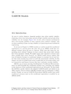
8 The sample average for daily return is almost zeromean(r)[1] on average, you can not make (or lose) money by using the buying yesterday and selling today strategy for this stock inthis return predictable? First, the Ljung-Box test indicates that the return is like a whitenoise, which is serially uncorrelated and (r, lag = 1, type="Ljung")Box-Ljung testdata: rX-squared = , df = 1, p-value = the p-value is , greater than So we cannot rejectthe null that the series is a white return predictable? Next, the AR(1) model applied to the price isarima(x = r, order = c(1, 0, 0))Coefficients:ar1 both the intercept and autoregressive coefficients areinsignificant The last evidence for unpredictable return is its ACF function33 ACF of r34 How about squared returnSquared We see that volatile periods are clustered; so volatility in thisperiod will affect next period s volatility. The Ljung-Box test applied to squared return is> (r2, lag = 1, type="Ljung")Box-Ljung testdata: r2X-squared = , df = 1, p-value = we can reject the null hypothesis of squared return beingwhite noise at 1% level (the p-value is , less than )36 ACF of squared r237 ACF of squared returnWe can see significant autocorrelation at the first and 15th lags.

9 Thisis evidence that the squared return is (1) Model: OLS estimation We first try OLS estimation of the ARCH(1) model, whichessentially regressesr2tonto its first lag> arima(x = r2, order = c(1, 0, 0), method = "CSS")Coefficients:ar1 +00 Both the intercept and arch coefficient are (1) Model: ML estimationgarch(x = r, order = c(0, 1))Coefficient(s):Estimate Std. Error t value Pr(>|t|)a0 <2e-16 **a1 *Diagnostic Tests:Jarque Bera Testdata: ResidualsX-squared = , df = 2, p-value < testdata: = , df = 1, p-value = The algorithm converges! The ARCH coefficient estimated by ML is , close to theOLS estimate The Jarque Bera Test rejects the null hypothesis that theconditional distribution of the return is normal distribution The Box-Ljung test indicates that the ARCH(1) model isdynamically adequate with white noise (1,1) Modelgarch(x = r, order = c(1, 1))Coefficient(s):Estimate Std. Error t value Pr(>|t|)a0 **a1 *b1 Tests:Jarque Bera Testdata: ResidualsX-squared = , df = 2, p-value < testdata: = , df = 1, p-value = The algorithm converges!

10 The GARCH coefficient is , and is insignificant. The ARCH coefficient is , similar to the ARCH(1) model Becausea1 +b1 1 the squared return series is stationary(there is no IGARCH effect for WMT stock) Overall, we conclude that the return of Walmart stock pricefollows an ARCH(1)