Transcription of Lecture1.TransformationofRandomVariables
1 1 Lecture 1. Transformation of random VariablesSuppose we are given a random variableXwith densityfX(x). We apply a functiongto produce a random variableY=g(X). We can think ofXas the input to a blackbox ,andYthe output. We wish to find the density or distribution function the technique for the example in Figure e-x1/2-1f (x)x-axisXYyX-Sqrt[y]Sqrt[y]Y = X2 Figure ,and thenfYby haveFY(y)=0fory<0. Ify 0 ,thenP{Y y}=P{ y x y}.Case y 1 (Figure ). ThenFY(y)=12 y+ y012e xdx=12 y+12(1 e y).1/2-1x-axis-Sqrt[y]Sqrt[y]f (x)XFigure >1 (Figure ). ThenFY(y)=12+ y012e xdx=12+12(1 e y).The density ofYis 0 fory<0 and21/2-1x-axis-Sqrt[y]Sqrt[y]f (x)X1'Figure (y)=14 y(1 +e y),0<y<1;fY(y)=14 ye y,y> Figure for a sketch offYandFY. (You can takefY(y) to be anything you like aty= 1 because{Y=1}has probability zero.)yf (y)Y1'yF (y)Y112y+12(1-e-y)12+12(1-e-y)'Figure ,and thenFYby integration; seeFigure We havefY(y)|dy|=fX( y)dx+fX( y)dx; we write|dy|because proba-bilities are never negative.
2 ThusfY(y)=fX( y)|dy/dx|x= y+fX( y)|dy/dx|x= ywithy=x2, dy/dx=2x ,sofY(y)=fX( y)2 y+fX( y)2 y.(Note that| 2 y|=2 y.) We havefY(y) = 0 fory<0 ,and:Case <y<1 (see Figure ).fY(y)=(1/2)e y2 y+1/22 y=14 y(1 +e y).3 Case >1 (see Figure ).fY(y)=(1/2)e y2 y+0=14 ye yas -yFigure distribution function method generalizes to situations where we have a single out-put but more than one input. For example ,letXandYbe independent ,each uniformlydistributed on [0,1]. The distribution function ofZ=X+YisFZ(z)=P{X+Y z}= x+y zfXY(x,y)dxdywithfXY(x,y)=fX(x)fY(y) by independence. NowFZ(z)=0forz<0 andFZ(z)=1forz>2 (because 0 Z 2).Case z 1 ,thenFZ(z) is the shaded area in Figure ,which isz2 z 2 ,thenFZ(z) is the shaded area in Figure ,which is 1 [(2 z)2/2].Thus (see Figure )fZ(z)= z,0 z 12 z1 z LetX,Y,Zbe independent ,identically distributed (from now on ,abbreviated iid) random variables ,each with densityf(x)=6x5for 0 x 1 ,and 0 elsewhere.
3 Findthe distribution and density functions of the maximum ofX, LetXandYbe independent ,each with densitye x,x 0. Find the distribution (fromnow on ,an abbreviation for Find the distribution or density function ) ofZ= A discrete random variableXtakes valuesx1,..,xn ,each with probability 1/n. LetY=g(X) wheregis an arbitrary real-valued function. Express the probability functionofY(pY(y)=P{Y=y}) in terms ofgand +y = z1 z 22-z2-zFigures and (z)Z-112'zFigure A random variableXhas densityf(x)=ax2on the interval [0,b]. Find the densityofY= TheCauchy densityis given byf(y)=1/[ (1 +y2)] for all realy. Show that one wayto produce this density is to take the tangent of a random variableXthat is uniformlydistributed between /2 and 2. JacobiansWe need this idea to generalize the density function method to problems where there arekinputs andkoutputs ,withk 2.
4 However ,if there arekinputs andj<koutputs,often extra outputs can be introduced ,as we will see later in the The SetupLetX=X(U,V),Y=Y(U,V). Assume a one-to-one transformation ,so that we cansolve (X,Y),V=V(X,Y). Look at Figure Ifuchangesbyduthenxchanges by ( x/ u)duandychanges by ( y/ u)du. Similarly ,ifvchangesbydvthenxchanges by ( x/ v)dvandychanges by ( y/ v)dv. The small rectangle intheu vplane corresponds to a small parallelogram in thex yplane (Figure ) ,withA=( x/ u, y/ u,0)duandB=( x/ v, y/ v,0)dv. The area of the parallelogramis|A B|andA B= IJK x/ u y/ u0 x/ v y/ v0 dudv= x/ u x/ v y/ u y/ v dudvK.(A determinant is unchanged if we transpose the matrix , ,interchange rows andcolumns.) x u du y u duxyuvdudvRFigure Definition and DiscussionTheJacobianof the transformation isJ= x/ u x/ v y/ u y/ v ,written as (x,y) (u,v).
5 6 Thus|A B|=|J| {(X,Y) S}=P{(U,V) R} ,in other words ,fXY(x,y) times the area ofSisfUV(u,v) times the area (x,y)|J|dudv=fUV(u,v)dudvandfUV(u,v)=fXY (x,y) (x,y) (u,v) .The absolute value of the Jacobian (x,y)/ (u,v) gives a magnification factor for areain going fromu vcoordinates tox ycoordinates. The magnification factor going theother way is| (u,v)/ (x,y)|. But the magnification factor fromu vtou vis 1 ,sofUV(u,v)=fXY(x,y)| (u,v)/ (x,y)|.In this formula ,we must substitutex=x(u,v),y=y(u,v) to express the final result interms three dimensions ,a small rectangular box with volumedudvdwcorresponds to aparallelepiped inxyzspace ,determined by vectorsA= x u y u z u du, B= x v y v z v dv, C= x w y w z w volume of the parallelepiped is the absolute value of the dot product ofAwithB C,and the dot product can be written as a determinant with rows (or columns)A,B,C.
6 Thisdeterminant is the Jacobian ofx,y,zwith respect tou,v,w[written (x,y,z)/ (u,v,w)],timesdudvdw. The volume magnification fromuvwtoxyzspace is| (x,y,z)/ (u,v,w)|and we havefUVW(u,v,w)=fXYZ(x,y,z)| (u,v,w)/ (x,y,z)|withx=x(u,v,w),y=y(u,v,w),z=z(u, v,w).The Jacobian technique extends to higher dimensions. The transformation formula isa natural generalization of the two and three-dimensional cases:fY1Y2 Yn(y1,..,yn)=fX1 Xn(x1,..,xn)| (y1,..,yn)/ (x1,..,xn)|where (y1,..,yn) (x1,..,xn)= y1 x1 y1 yn x1 yn xn .To help you remember the formula ,thinkfY(y)dy=fX(x) ATypical ApplicationLetXandYbe independent ,positive random variables with densitiesfXandfY ,and letZ=XY. We find the density ofZby introducing a new random variableW ,as follows:Z=XY, W=Y(W=Xwould be equally good). The transformation is one-to-one because we can solveforX,Yin terms ofZ,WbyX=Z/W,Y=W.
7 In a problem of this type ,we must alwayspay attention to the range of the variables:x>0,y >0 is equivalent toz>0,w> (z,w)=fXY(x,y)| (z,w)/ (x,y)|x=z/w,y=wwith (z,w) (x,y)= z/ x z/ y w/ x w/ y = yx01 = (z,w)=fX(x)fY(y)w=fX(z/w)fY(w)wand we are left with the problem of finding the marginal density from a joint density:fZ(z)= fZW(z,w)dw= 01wfX(z/w)fY(w) The joint density of two random variablesX1andX2isf(x1,x2)=2e x1e x2,where 0<x1<x2< ;f(x1,x2) = 0 elsewhere. Consider the transformationY1=2X1,Y2=X2 X1. Find the joint density ofY1andY2 ,and conclude thatY1andY2are Repeat Problem 1 with the following new data. The joint density is given byf(x1,x2)=8x1x2,0<x1<x2<1;f(x1,x2) = 0 elsewhere;Y1=X1/X2,Y2= Repeat Problem 1 with the following new data. We now have three iid random variablesXi,i=1,2,3 ,each with densitye x,x>0.
8 The transformation equations are givenbyY1=X1/(X1+X2),Y2=(X1+X2)/(X1+X2+X 3),Y3=X1+X2+ ,find the joint density of theYiand show thatY1,Y2andY3are on the Problem SetIn Problem 3 ,notice thatY1Y2Y3=X1,Y2Y3=X1+X2 ,soX2=Y2Y3 Y1Y2Y3,X3=(X1+X2+X3) (X1+X2)=Y3 (x,y)=g(x)h(y) for allx,y ,thenXandYare independent ,becausef(y|x)=fXY(x,y)fX(x)=g(x)h(y)g(x ) h(y)dy8which does not depend onx. The set of points whereg(x) = 0 (equivalentlyfX(x)=0)can be ignored because it has probability zero. It is important to realize that in thisargument , for allx,y means thatxandymust be allowed to vary independently of eachother ,so the set of possiblexandymust be of the rectangular forma<x<b,c<y<d.(The constantsa,b,c,dcan be infinite.) For example ,iffXY(x,y)=2e xe y,0<y<x,and 0 elsewhere ,thenXandYarenotindependent. Knowingxforces 0<y<x ,so theconditional distribution ofYgivenX=xcertainly depends onx.
9 Note thatfXY(x,y)isnota function ofxalone times a function ofyalone. We havefXY(x,y)=2e xe yI[0<y<x]where theindicatorIis 1 for 0<y<xand 0 Jacobian problems ,pay close attention to the range of the variables. For example ,inProblem 1 we havey1=2x1,y2=x2 x1 ,sox1=y1/2,x2=(y1/2) +y2. From theseequations it follows that 0<x1<x2< is equivalent toy1>0,y2> 3. Moment-Generating DefinitionThemoment-generating functionof a random variableXis defined byM(t)=MX(t)=E[etX]wheretis a real number. To see the reason for the terminology ,note thatM(t) is theexpectation of 1 +tX+t2X2/2! +t3X3/3! + .If n=E(Xn) ,then-th moment ofX,and we can take the expectation term by term ,thenM(t)=1+ 1t+ 2t22!+ + ntnn!+ .Since the coefficient oftnin the Taylor expansion isM(n)(0)/n! ,whereM(n)is then-thderivative ofM ,we have n=M(n)(0). The Key TheoremIfY= ni=1 XiwhereX1.
10 ,Xnare independent ,thenMY(t)= ni=1 MXi(t).Proof. First note that ifXandYare independent ,thenE[g(X)h(Y)] = g(x)h(y)fXY(x,y) (x,y)=fX(x)fY(y) ,the double integral becomes g(x)fX(x)dx h(y)fY(y)dy=E[g(X)]E[h(Y)]and similarly for more than two random variables. Now ifY=X1+ +Xnwith theXi s independent ,we haveMY(t)=E[etY]=E[etX1 etXn]=E[etX1] E[etXn]=MX1(t) MXn(t). The Main ApplicationGiven independent random variablesX1,..,Xnwith densitiesf1,..,fnrespectively,find the density ofY= ni= 1. ComputeMi(t) ,the moment-generating function ofXi ,for 2. ComputeMY(t)= ni=1Mi(t).Step 3. FromMY(t) findfY(y).This technique is known as atransform method. Notice that the moment-generatingfunction and the density of a random variable are related byM(t)= etxf(x) by swe have aLaplace transform ,and withtreplaced byitwe have aFourier transform.