Transcription of Mathematica Tutorial: Differential Equation Solving With ...
1 Wolfram Mathematica Tutorial CollectionDIFFERENTIAL Equation Solving WITH DSOLVEFor use with Wolfram Mathematica and later. For the latest updates and corrections to this manual: visit For information on additional copies of this documentation: visit the Customer Service website at or email Customer Service at Comments on this manual are welcomed at: Content authored by: Devendra Kapadia Printed in the United States of America. 15 14 13 12 11 10 9 8 7 6 5 4 3 2 2008 Wolfram Research, Inc. All rights reserved. No part of this document may be reproduced or transmitted, in any form or by any means, electronic, mechanical, photocopying, recording or otherwise, without the prior written permission of the copyright holder. Wolfram Research is the holder of the copyright to the Wolfram Mathematica software system ("Software") described in this document, including without limitation such aspects of the system as its code, structure, sequence, organization, look and feel, programming language, and compilation of command names.
2 Use of the Software unless pursuant to the terms of a license granted by Wolfram Research or as otherwise authorized by law is an infringement of the copyright. Wolfram Research, Inc. and Wolfram Media, Inc. ("Wolfram") make no representations, express, statutory, or implied, with respect to the Software (or any aspect thereof), including, without limitation, any implied warranties of merchantability, interoperability, or fitness for a particular purpose, all of which are expressly disclaimed. Wolfram does not warrant that the functions of the Software will meet your requirements or that the operation of the Software will be uninterrupted or error free. As such, Wolfram does not recommend the use of the software described in this document for applications in which errors or omissions could threaten life, injury or significant loss. Mathematica , MathLink, and MathSource are registered trademarks of Wolfram Research, Inc.
3 J/Link, MathLM, .NET/Link, and webMathematica are trademarks of Wolfram Research, Inc. Windows is a registered trademark of Microsoft Corporation in the United States and other countries. Macintosh is a registered trademark of Apple Computer, Inc. All other trademarks used herein are the property of their respective owners. Mathematica is not associated with Mathematica Policy Research, Inc. ContentsIntroduction to Differential Equation Solving with DSolve ..1 Classification of Differential Equations ..7 Ordinary Differential Equations (ODEs) ..11 Overview of ODEs ..11 First-Order ODEs ..12 Linear Second-Order ODEs ..24 Nonlinear Second-Order ODEs ..33 Higher-Order ODEs ..36 Systems of ODEs ..42 Lie Symmetry Methods for Solving Nonlinear ODEs ..50 partial Differential Equations (PDEs) ..55 Introduction to PDEs ..55 First-Order PDEs ..56 Second-Order PDEs ..66 Differential -Algebraic Equations (DAEs).
4 70 Introduction to DAEs ..70 Examples of DAEs ..71 Initial and Boundary Value Problems ..76 Introduction to Initial and Boundary Value Problems ..76 Linear IVPs and BVPs ..77 Nonlinear IVPs and BVPs ..82 IVPs with Piecewise Coefficients ..85 Working with DSolve~A User s Guide ..89 Introduction ..89 Setting Up the Problem ..90 Verification of the Solution ..94 Plotting the Solution ..98 The GenerateParameters Options ..102 Symbolic Parameters and Inexact Quantities ..104Is the Problem Well-Posed? ..108 References ..111 Introduction to Differential Equation Solving with DSolveThe Mathematica function DSolve finds symbolic solutions to Differential equations. (The Mathe-matica function NDSolve, on the other hand, is a general numerical Differential equationsolver.) DSolve can handle the following types of equations: Ordinary Differential Equations (ODEs), in which there is a single independent variable t andone or more dependent variables xiHtL.
5 DSolve is equipped with a wide variety of techniquesfor Solving single ODEs as well as systems of ODEs. partial Differential Equations (PDEs), in which there are two or more independent variablesand one dependent variable. Finding exact symbolic solutions of PDEs is a difficult problem,but DSolve can solve most first-order PDEs and a limited number of the second-order PDEsfound in standard reference books. Differential -Algebraic Equations (DAEs), in which some members of the system are differen-tial equations and the others are purely algebraic, having no derivatives in them. As withPDEs, it is difficult to find exact solutions to DAEs, but DSolve can solve many examples ofsuch systems that occur in @eqn,y@xD,xDsolve a Differential Equation for y@ @ a system of Differential equations for yi@xDFinding symbolic solutions to ordinary Differential returns results as lists of rules. This makes it possible to return multiple solutions to anequation.
6 For a system of equations, possibly multiple solution sets are grouped together. Youcan use the rules to substitute the solutions into other finds the general solution for the given ODE. A rule for the function that satisfies the Equation is returned. In[1]:=DSolve@8y'@xD y@xD<, y@xD, xDOut[1]=99y@xD xC@1D==You can pick out a specific solution by using . (ReplaceAll).In[2]:=y@xD . DSolve@8y'@xD y@xD<, y@xD, xDOut[2]=9 xC@1D=A general solution contains arbitrary parameters C@iD that can be varied to produce particularsolutions for the Equation . When an adequate number of initial conditions are specified, DSolvereturns particular solutions to the given , the initial condition y@0D==1 is specified, and DSolve returns a particular solution for the [3]:=sol=DSolve@8y'@xD y@xD, y@0D 1<, y@xD, xDOut[3]=99y@xD x==This plots the solution. ReplaceAll ( .) is used in the Plot command to substitute the solution for @y@xD.
7 Sol,8x,-3, 2<DOut[4]=-3-2-1121234567 DSolve@eqn,y,xDsolve a Differential Equation for y as a pure a system of Differential equations for the pure func-tions yi Finding symbolic solutions to ordinary Differential equations as pure the second argument to DSolve is specified as y instead of y@xD, the solution is returned asa pure function. This form is useful for verifying the solution of the ODE and for using the solu-tion in further work. More details are given in "Setting Up the Problem".2 Differential Equation Solving with DSolveThe solution to this Differential Equation is given as a pure [5]:=eqn=8y'@xD y@xD^2, y@0D 1<;sol=DSolve@eqn, y, xDOut[6]=::y FunctionB8x<,11-xF>>This verifies the [7]:=eqn . solOut[7]=88 True, True<<This solves a system of ODEs. Each solution is labeled according to the name of the function (here, x and y), making it easier to pick out individual [8]:=eqns=8Ht^2+1L*x'@tD -t*x@tD+y@tD-Sign@tD,Ht^2+1L*y'@tD -x@tD-t*y@tD+t*UnitStep@tD, x@0D -1 2, y@0D 2<;sol=DSolve@eqns,8x, y<, tDOut[9]=::x FunctionB8t<,-1+4 t+2 ArcTan@tDt 0-tTrue+2 t12 LogA1+t2Et 00 True2I1+t2MF,y FunctionB8t<,4+t-2 t ArcTan@tDt 0-tTrue+212 LogA1+t2Et 00 True2I1+t2MF>>This substitutes a random value for the independent variable and shows that the solutions are correct at that [10]:=eqns.
8 Sol .8t RandomReal@D<Out[10]=88 True, True, True, True<<This plots the [11]:=Plot@8x@tD . sol, y@tD . sol<,8t,-10, 10<DOut[11]=-10-5510-112 DSolve@eqn,u@x,yD,8x,y<Dsolve a partial Differential Equation for u@x,yDFinding symbolic solutions to partial Differential general solutions to ordinary Differential equations involve arbitrary constants, generalsolutions to partial Differential equations involve arbitrary functions. DSolve labels these arbi-trary functions as Equation Solving with DSolve 3 While general solutions to ordinary Differential equations involve arbitrary constants, generalsolutions to partial Differential equations involve arbitrary functions. DSolve labels these arbi-trary functions as is the general solution to a linear first-order PDE. In the solution, C@1D labels an arbitrary function of -x+yx [12]:=eqn=x^2*D@u@x, yD, xD+y^2*D@u@x, yD, yD-Hx+yL*u@x, yD;sol=DSolve@eqn 0, u,8x, y<DOut[13]=::u FunctionB8x, y<,-x y C@1DB-x+yx yFF>>This obtains a particular solution to the PDE for a specific choice of @x, yD.
9 Sol@@1DD .8C@1D@t_D Sin@t^2D+Ht 10L<Out[14]=-x y-x+y10 x y+SinBH-x+yL2x2y2 FHere is a plot of the surface for this [15]:=Plot3D@fn,8x,-5, 5<,8y,-5, 5<DOut[15]=DSolve can also solve Differential -algebraic equations. The syntax is the same as for a systemof ordinary Differential solves a [16]:=eqns=8f''@xD==g@xD, f@xD+g@xD==3 Sin@xD, f@PiD==1, f'@PiD==0<;sol=DSolve@eqns,8f, g<, xDOut[17]=::f FunctionB8x<,12H-2 Cos@xD+3pCos@xD-3 x Cos@xD+3 Sin@xDLF,g FunctionB8x<,12H2 Cos@xD-3pCos@xD+3 x Cos@xD+3 Sin@xDLF>>This verifies the Differential Equation Solving with DSolveThis verifies the [18]:=Simplify@eqns . solDOut[18]=88 True, True, True, True<<A plot of the solutions shows that their sum satisfies the algebraic relation f@xD+g@xD 3 @8f@xD . sol, g@xD . sol, f@xD+g@xD . sol<,8x,-5, 5<DOut[19]=-4-224-55 Goals of Differential Equation Solving with DSolve TutorialsThe design of DSolve is modular: the algorithms for different classes of problems work indepen-dently of one another.
10 Once a problem has been classified (as described in "Classification ofDifferential Equations"), the available methods for that class are tried in a specific sequenceuntil a solution is obtained. The code has a hierarchical structure whereby the solution of com-plex problems is reduced to the solution of relatively simpler problems, for which a greatervariety of methods is available. For example, higher-order ODEs are typically solved by reduc-ing their order to 1 or 2. The process described is done internally and does not require any intervention from the this reason, these tutorials have the following basic goals. To provide enough information and tips so that users can pose problems to DSolve in themost appropriate form and apply the solutions in their work. This is accomplished through asubstantial number of examples. A summary of this information is given in "Working withDSolve".