Transcription of MATHEMATICS FOR ENGINEERING DIFFERENTIATION …
1 1 MATHEMATICS FOR ENGINEERING DIFFERENTIATION TUTORIAL 1 - BASIC DIFFERENTIATION This tutorial is essential pre-requisite material for anyone studying mechanical ENGINEERING . This tutorial uses the principle of learning by example. The approach is practical rather than purely mathematical and may be too simple for those who prefer pure maths. Calculus is usually divided up into two parts, integration and DIFFERENTIATION . Each is the reverse process of the other. integration is covered in tutorial 1. On completion of this tutorial you should be able to do the following. Explain differential coefficients. Apply Newton s rules of DIFFERENTIATION to basic functions. Solve basic ENGINEERING problems involving DIFFERENTIATION . Define higher differential coefficients. Evaluate higher order differential coefficient. 2 DIFFERENTIATION 1.
2 DIFFERENTIAL COEFFICIENTS DIFFERENTIATION is the reverse process of integration but we will start this section by first defining a differential coefficient. Remember that the symbol means a finite change in something. Here are some examples. Temperature change T = T2 T1 Change in time t = t2 t1 Change in Angle = 2 1 Change in distance x = x2 x1 Change in velocity v = v2 v1 The symbol means a small but finite change in something such as T, t, , x, v and so on. Consider the following. The distance moved by an object is directly proportional to time t as shown on the graph. Figure 1 Velocity = Change in distance/change in time. v = x/ t This would be the same for a small change. v = x/ t = x/ t The ratio x/ t is the same as the ratio x/ t and the ratio is the gradient of the straight line. INFINITESIMALLY SMALL CHANGES d The symbol d is used to denote a change that is infinitesimally small.
3 On our graph the ratios are all the same and equal to the velocity. This value is the same at any point on a straight-line graph. v = dx/dt = x/ t = x/ t. This ratio holds true even when the changes approach zero. 3 Now consider the case when acceleration occurs and the velocity is changing. The graph of x against t is an upwards curve. Figure 2 We can no longer say v = x/ t but v = x/ t might give a reasonable approximation if it is possible to measure the small changes. The result of evaluating v = x/ t would give the velocity at the time the measurements were made. At some other time the value would be different. If we were able to take our measurements over smaller and smaller intervals, the velocity would become the instantaneous velocity. When the value of t tends to zero we would write t 0. We would say that in the limit, as t 0, the ratio x/ t becomes the differential coefficient (the true ratio) and we write it as dx/dt.
4 It should be obvious now that the differential coefficient is the rate of change of one variable with another and is also the gradient of the graph at a given point. v = dx/dt gives the precise velocity at an instant in time but of course we could not find it by measuring dx and dt. Newton s calculus method allows us to find these differential coefficients if we have a mathematical equation linking the two variables. When a body accelerates at a m/s2 the formula relating distance and time is x = a t2/2. The velocity is the ratio dx/dt and it may be found at any moment in time by applying Newton s rules for DIFFERENTIATION . Remember DIFFERENTIATION gives the gradient of the function. 4 2. NEWTON S METHOD DIFFERENTIATION OF AN ALGEBRAIC EXPRESSION The equation x = a t2/2 is an example of an algebraic equation. In general we use x and y and a general equation may be written as y = Cxn where C is a constant and n is a power or index.
5 The rule for differentiating is : dy/dx = Cnx (n-1) or dy = Cnx (n-1) dx Note that integrating returns the equation back to its original form. DERIVATION For those who want to know where this comes from here is the derivation. Consider to points A and B on a curve of y = Cxn Join AB with a straight line and the gradient of the line is approximately the gradient at point P. The closer A and B are the more accurate this becomes. Gradient at P BC/AC h is the difference between the value of x at B and A. =lim 0 ( ) ( ) dydx=lim 0 ( + ) ( ) =lim 0 ( + ) dydx=lim 0 1+ =lim 0 1+ 1 If we expand 1+ we get a series 1+ + 2+ 3+ =lim 0 1+ + 2+ 3+ 1 =lim 0 + 2+ 3+ divide out the h =lim 0 + 2+ 2 3+ Put h = 0 and = 1 5 DIFFERENTIATING A CONSTANT.
6 Consider the equation y = a xn. When n = 0 this becomes y = a x0 = a (the constant). (Remember that anything to the power of zero is unity). Using the rule for DIFFERENTIATION dy/dx = anx 0-1 = a (0)x-1 = 0 The constant disappears when integrated. This explains why, when you do integration without limits, you must add on a constant that might or might not have been present before you differentiated. It is important to remember that: A constant disappears when differentiated. WORKED EXAMPLE Differentiate the function x = 3 t2/2 with respect to t and evaluate it when t = 2. SOLUTION 6dtdx find we2 t Putting3t2(2)(3)tdtdx 23tx122 WORKED EXAMPLE Differentiate the function y = 4 + x2 with respect to y and evaluate it when y = 5. SOLUTION 10dxdy find we5 y Putting2x2x0dxdy x4y122 6 WORKED EXAMPLE Differentiate the function z = 2y4 with respect to y and evaluate it when y = 3.
7 SOLUTION 216dydz find we3 y Putting8y2)(4)x(dydz 2yz3144 WORKED EXAMPLE Differentiate the function p = 2q3 + 3q5 +5 with respect to q and evaluate it when q = 2. SOLUTION 26424024dqdpget we2q p utting15q6q 0(5)(3)q(3)(2)qdqdp53q2qp42151353 WORKED EXAMPLE The equation linking distance and time is x = 4t + at2 where a is the acceleration. Find the velocity at time t = 4 seconds given a = m/s2. SOLUTION x = 4t + at2 velocity = v = dx/dt = 4 + at = 4 +( )(4) = 10 m/s 7 SELF ASSESSMENT EXERCISE 1. Find the gradient of the function y = 2x - 5x7 when x = 2 (Answer -2238) 2. Find the gradient of the function p = 2q + 2q2 + 4q3 and evaluate when q = 3 (Answer 122) 3. Find the gradient of the function u = 2v2 + 4v4 and evaluate when v = 5 (Answer 2020) SELF ASSESSMENT EXERCISE 1. The electric charge entering a capacitor is related to time by the equation q = 3t2.
8 Determine the current (i = dq/dt) after 5 seconds. (30 Amp) 2. The angle radians turned by a wheel after t seconds from the start of measurement is found to be related to time by the equation = 1 t + t2 1 is the initial angular velocity (2 rad/s) and is the angular acceleration ( rad/s2). Determine the angular velocity ( = d /dt) 8 seconds from the start. (6 rad/s) 8 OTHER STANDARD FUNCTIONS For other common functions the differential coefficients may be found from the look up table below. kxkx12akedxdy aeyx1xdxdy ln(ax)yatan(ax)adxdy tan(ax)yasin(ax)dxdy cos(ax)yacos(ax)dxdy sin(ax)y WORKED EXAMPLE The distance moved by a mass oscillating on a spring is given by the equation: x = 5 cos (8 t) mm. Find the distance and velocity after seconds. SOLUTION At seconds x = 5 cos ( ) = mm v = dx/dt = -40 sin (8t) = -40 sin ( ) = mm/s Note that your calculator must be in radian mode when looking up sine and cosine values.
9 WORKED EXAMPLE The distance moved by a mass is related to time by the equation : x = 20e mm. Find the distance and velocity after seconds. SOLUTION At seconds x = 20e = 20e = mm v = dx/dt = (20)( ) e = 10 e = mm/s 9 SELF ASSESSMENT EXERCISE 1. If the current flowing in a circuit is related to time by the formula i = 4sin(3t), find the rate of change of current after seconds. ( A/s) 2. The voltage across a capacitor C when it is being discharged through a resistance R is related to time by the equation v = 4e-t/T where T = is a time constant and T = RC. Find the voltage and rate of change of voltage after seconds given R = 10 k and C = 20 F. ( V and V/s ) 3. The voltage across a capacitor C when it is being charged through a resistance R is related to time by the equation v = 4 - 4e-t/T where T = is a time constant and T = RC.
10 Find the voltage and rate of change of voltage after seconds given R = 10 k and C = 20 F. ( V and V/s ) 4. The distance moved by a mass is related to time by the equation : x = 17e mm. Find the distance and velocity after seconds. ( mm and mm/s) 5. The angle turned by a simple pendulum is given by the equation: = sin (6 t) mm. Find the angle and angular velocity (d /dt) after seconds. ( radian and rad/s) 10 3. HIGHER ORDER DIFFERENTIALS Consider the function y = x3. The graph looks like this. Figure 3 The gradient of the graph at any point is dy/dx =3x2. This may be evaluated for any value of x. If we plot dy/dx against x we get the following graph. Figure 4 This graph is also a curve. We may differentiate again to find the gradient at any point. This is the gradient of the gradient. We write it as follows. 6xdxyddxdxdyd22 The graph is a straight line as shown with a gradient of 6 at all points.