Transcription of MATHEMATICS FOR ENGINEERING STATISTICS …
1 1 MATHEMATICS FOR ENGINEERING STATISTICS TUTORIAL 1 BASICS OF STATISTICAL data This tutorial is useful to anyone studying ENGINEERING . It uses the principle of learning by example. On completion of this tutorial you should be able to do the following. Explain the use of raw data . Present data as frequency polygons, bar graphs and histograms. Explain and find the mean and median values. Explain and plot ogives. Explain and find quartiles. Explain and find the standard deviation and variance for grouped and ungrouped data . 2 1. INTRODUCTION STATISTICS are used to help us analyse and understand the performance and trends in various areas of work. These might be financial trends, things to do with the population or things to do with manufacturing.
2 Often we wish to present information visually with easily understood graphics and so a variety of graphs and charts are used for this purpose. Here is an example of a PIE CHART and a BAR CHART showing the number of parliamentary seats won by main political parties at the 2001 British general election. The number of MPs elected must be a round or whole number so the raw data is exact. When presenting other forms of data this is not the case as explained in the following section. 2. RAW data Let s use an example to get started. Consider a set of STATISTICS compiled for the height of children of age 10. First we would compile a table of heights. This would be the raw data . Note that the larger the sample we take, the more meaningful the results will be.
3 Suppose we measure the heights to an accuracy of m. This is the table of raw data for 10 year old children Sample 1 2 3 4 5 6 7 8 9 10 11 12 Height (m) Sample 13 14 15 16 17 Height (m) 3. RANKED data If the raw data is rearranged from shortest to tallest we have the ranked data . Sample number 1 2 3 4 5 6 7 8 9 10 11 12 13 Height (m) Sample number 14 15 16 17 Total Height (m) data presented in this form is also called DISCRETE data because we jump from one value to another in steps, in this case steps of m. 3 4. CLASS or BANDS If we used exact measurements of heights, it is unlikely we would find two children exactly the same height so we round off the values.
4 This causes problems as we shall see. When handling large numbers of samples, we end up with huge lists of data so to simplify the table we create bands or classes within which the rounded measurements fall. The more we round off the values, the more likely it becomes that we will find more than one in a given class. The number of children within each class is the frequency. Next we would have to go through the laborious task of counting how many there are in each class. If we found a child with a height exactly on the edge of the class edge, we might decide to allocate a half to each class on either side resulting in frequency values that are not whole numbers. The result is a FREQUENCY DISTRIBUTION TABLE.
5 Height - - - - - Mid Point or MARK Freq. 2 5 6 3 1 5. GRAPHS If we plot frequency vertically against height horizontally, we get a frequency distribution graph and this can be drawn in different ways. The values plotted are the mid point values called the MARK. These plots simply tell us the numbers in each class by the mark. If we want to illustrate the width of the band we use a HISTOGRAM. Notice that the mid point of each band is the MARK. The boxes are drawn between the CLASS LIMITS. Because the heights were rounded off to m the limits are either side of the CLASS BOUNDARY and the class boundary is the exact dividing line between each class.
6 The width of the band from mark to mark or boundary to boundary is the CLASS INTERVAL. In this example the interval is The area of the bars on histograms usually represents the frequency so the vertical plot is frequency density. This found by dividing the frequency by the width of the bar. Notice that the points are drawn for the middle of the band. 4 6. MEAN This is one of the more common STATISTICS you will see and it's easy to compute. All you have to do is add up all the values in a set of data and then divide that sum by the number of values in the dataset. For our example, let the height be represented by the variable x and the frequency be f. Sample number 1 2 3 4 5 6 7 8 9 10 11 12 13 Height (m) Sample number 14 15 16 17 Total Height (m) The mean value is denoted x and x= = m We can do this a bit more simply using the frequency distribution table.
7 X (mid pt) f. 2 5 6 3 1 total f x The mean value is x= = m. This is not quite as accurate as the previous answer because the values have been taken at the mid point of the band. 7. MEDIAN Whenever you see words like, "the average person ..", or "the average income of .. you don't always want to know the mean. Often you want to know the about the one in the middle. That's the median. Again, this statistic is easy to determine because the median literally is the value in the middle. In order to find it, you just line up the values in your set of data from largest to smallest. The one in the dead-centre is your median. Our table would look like this. Sample number 1 2 3 4 5 6 7 8 9 10 11 12 13 Height (m) Sample number 14 15 16 17 Total Height (m) The mid point in the table is point number 9 so the median value is m.
8 If we had an even number of samples, say 18, then there would be two values in the middle and we should average the two to get the median. 5 8. MODE The mode is the most frequently occurring value. In the example repeated below, this will be the class with a mark of since there are six in this group. x (mark) f. 2 5 6 3 1 total f x It is quite possible that the mode is not unique because the same maximum figure could occur more than once the distribution. If we don't have grouped data , there is no mode unless several occur at the same precise height. This leads us on to the next section. 9. OGIVE and QUARTILES If we add a new row to our data showing the accumulative frequency and plot the data against it, we get a different sort of graph called an OGIVE that makes it easier to spot the median.
9 Let s add a new row to our frequency distribution table containing the cumulative frequency. We can plot the same data using bands of m. We plot the upper limit of each band so that each frequency shows how many children are either shorter or taller than that value. The table to plot is as follows. The vertical scale is usually turned divided into four quarters giving the projected points Q1, Q2 and Q3 as shown. The Q2 corresponds to the median. x (upper point) Total f. 2 5 6 3 1 n =17 f x cum. f 2 7 13 16 17 Q1 is called the lower Quartile and Q3 the upper Quartile. The range between them is called the inter quartile range and this can be divided into two parts called the semi-inter-quartile.
10 These tell us something about how the samples are spread around the median but a better method of doing this is to use the standard deviation. Any range corresponding to a change of 1% is called a percentile. Q1 is the 25th percentile, Q2 the 50th and Q3 the 75th. 6 WORKED EXAMPLE A company manufactures steel bars of nominal diameter 20 mm and cuts them into equal lengths. The diameter of each length is measured at the middle for the purpose of quality control. The results for 20 bars are given below. Produce a frequency distribution table using bands of mm. Calculate the mean of the samples. Draw a histogram. Plot the Ogive. Determine the median, mode, upper and lower quartiles and the semi- inter-quartile.