Transcription of May 1, 2007
1 NotesOnR0 James Holland Jones Department of Anthropological SciencesStanford UniversityMay 1, 20071 The Basic Reproduction Number in a NutshellThe basic reproduction number,R0, is defined as the expected number of secondary casesproduced by a single (typical) infection in a completely susceptible population. It is importantto note thatR0is a dimensionless number and not a rate, which would have units of time authors incorrectly callR0the basic reproductive rate. We can use the fact thatR0is a dimensionless number to help us in calculating (infectioncontact) (contacttime) (timeinfection)More specifically:R0= c d(1)where is the transmissibility ( , probability of infection given contact between a suscepti-ble and infected individual), cis the average rate of contact between susceptible and infectedindividuals, anddis the duration of The SIR Epidemic ModelIt is pretty clear how we calculateR0given information on transmissibility, contact rates, andthe expected duration of infection.
2 But how do we know that this quantity defines the epidemicthreshold of a particular infection? To understand this, we need to formulate an epidemic model we use is called an SIR model, where SIR stands for Susceptible-Infected-Removed. For simplicity, we will deploy several (closed) population size,N Correspondence Address: Department of Anthropological Sciences, Building 360, Stanford, CA 94305-2117;phone: 650-723-4824, fax: 650-725-9996; rates ( , transmission, removal rates) demography ( , births and deaths) populationA well-mixed population is one where any infected individual has a probability of contactingany susceptible individual that is reasonably well approximated by the average. This is oftenthe most problematic assumption, but is easily relaxed in more complex our closed population ofNindividuals, say thatSare susceptible,Iinfected, andRareremoved. Writes=S/N,i=I/N,r=R/Nto denote the fraction in each SIR model is then:dsdt= si(2)didt= si i(3)drdt= i(4)where = cand is known as the effective contact rate, is the removal rate.
3 By assumptionall rates are constant. This means that the expected duration of infection is simply the inverseof the removal rate:d= are the conditions for an epidemic? An epidemic occurs if the number of infectedindividuals increases, ,di/dt >0 si i >0 si > iAt the outset of an epidemic, nearly everyone (except the index case) is susceptible. So wecan say thats 1. Substitutings= 1, we arrive at the following inequality =R0>1 Since = candd= 1, we see that we have derived our expression forR0given inequation1. This little bit of mathematical trickery explains why we have that cumbersomephrase in a completely susceptible population tacked onto our definition Epidemic Thresholds in Structured Next Generation Matrix: Intuitive ApproachIfR0is the number of secondary infections produced by a single typical infection in a rarefiedpopulation, how do we define it when there are multiple types of infected individuals. For2example, what is atypicalinfection in a vector-borne disease like malaria?
4 What about asexually transmitted infection where there are large asymmetries in transmissibility (like HIV)?Or what about a multi-host pathogen like influenza?It turns out that there is a straightforward extension of the theory for structured epidemicmodels. The mathematics behind this theory is not especially difficult, but it does involve scaryGerman terms that are not familiar to the non-engineers in our midst. The key concept is thatwe now need to average the expected number of new infections over all possible infected that we have a system in which there are multiple discrete types of infected individ-uals ( , mosquitoes and humans; women and men; or humans, dogs, and chickens). We definethenext generation matrixas the square matrixGin which theijth element ofG,gij, is theexpected number of secondary infections of typeicaused by a single infected individual of typej, again assuming that the population of typeiis entirely susceptible. That is, each element ofthe matrixGis a reproduction number, but one where who infects whom is accounted we haveG, we are one step away fromR0.
5 The basic reproduction number is givenby thespectral radiusofG. The spectral radius is the also known as the dominant eigenvalueofG. The next generation matrix has a number of desirable properties from a mathematicalstandpoint. In particular, it is a non-negative matrix and, as such, it is guaranteed that therewill be a single, unique eigenvalue which is positive, real, and strictly greater than all the illustrative purposes, we will limit our discussion to the case where there are two classesof infected individual. The next generation matrix is thus 2 2. DefineG=[a bc d]The eigenvalues ofGare: =T2 (T /2)2 DwhereT=a+dis the trace andD=ad bcis the determinant of you have a sexually transmitted disease in a completely heterosexual population. Definefas the expected number of infected women andmas the expected number of infected mengiven contact with a single infected member of the opposite sex in a completely susceptiblepopulation. The next generation matrix isG=[0fm0]R0is thus mf.
6 It is worth noting that this is the geometric mean of the expected numberof female and male secondary Next Generation Matrix: More Formal ApproachA recent paper byHefferman et al.(2005) provides a nice readable introduction for calculatingR0in structured population models. The notation I use here follows their the next generation matrixG. It is comprised of two parts:FandV 1, whereF=[ Fi(x0) xj](5)andV=[ Vi(x0) xj](6)TheFiare the new infections, while theVitransfers of infections from one compartment the disease-free equilibrium the dominant eigenvalue of the matrixG=F V : SEIR EpidemicConsider a Susceptible-Exposed-Infected-Removed (SEIR) Epi-demic. This is an appropriate model for a disease where there is a considerable post-infectionincubation period in which the exposed person is not yet infectious. EIR ISI kE SFigure 1: State diagram for the SEIR model. is the effective contact rate, is the birth rate of susceptibles, is the mortality rate,kis the progression rate from exposed (latent) toinfected, is the removal simple SEIR model consists of a set of four differential equations: S= SI+ S(7) E= SI ( +k)E(8) I=kE ( + )I(9) R= I R(10)where is the effective contact rate, is the birth rate of susceptibles, is the mortality rate,kis the progression rate from exposed (latent) to infected, is the removal calculate the next generation matrix for the SEIR model, we need to enumerate thenumber of ways that (1) new infections can arise and (2) the number of ways that individualscan move between compartments.
7 There are two disease states but only one way to create newinfections:4V=( 00 0)(11)In contrast, there are various ways to move between the states:V=(0k+ + k)(12)R0is the leading eigenvalue of the matrixF V 1. This is reasonably straightforward tocalculate sinceF V 1is simply a 2 2 (k+ )( + )(13)It is interesting to note thatR0is also the product of the rate of production of (1) newexposures and (2) new infections, as it should What is a Generation?In demography,R0represents the ratio of total population size from the start to the end ofa generation, which is, roughly, the mean age of , whereris the in-stantaneous rate of increase of the population. So what is a generation in an epidemic model?Generations in epidemic models are the waves of secondary infection that flow from each previ-ous infection. So, the first generation of an epidemic is all the secondary infections that resultfrom infectious contact with the index case, who is of generation zero.
8 IfRidenotes the repro-duction number of theith generation, thenR0is simply the number of infections generated bythe index case, , generation zero. Now, these numbers are typically small and are thereforesusceptible to random sampling error. Consequently, we talk about expected ( , averaged overmany epidemics) numbers of secondary cases produced by generation zero. SeeDiekmann andHeesterbeek(2000) orHeesterbeek(2002) for a full discussion of this a schematic representation of an epidemic. The zeroth generation of theepidemic is the index case patient zero indicated in red. The number of secondary infectionsgenerated by the case in generation zero isR0= 3. In the first generation (blue),R1= 6/3 = second generation (cyan) hasR1= 12/6 = Will An Epidemic Infect Everyone?Will an epidemic, once it has taken off in a population, eventually infect everyone? In order toanswer this question, we want to know howichanges with respect to the fuel for the epidemic, thus divide equation4by 1 + s5We solve this equation by first multiplying both sides bydsdi= ( 1 + s)dsWe then integrate and do a little algebra, yieldinglog(s ) =R0(s 1)(14)This is an implicit equation fors , the number of susceptibles at the end of the >1, this equation has exactly two roots, only one of which lies in the interval (0,1).
9 Subtract log(s ) from both sides and we getR0(s 1) log(s ) = 0. Call the whole have different values for different values of log(s ). Only a couple of those willsatisfy equation14. log(s ) = 1 will always satisfy the requirement ofy= 0 (plug it in andsee!). WhenR0>1, the other solution toy= 0 is the actual value of the final size. This is theone we really care about. IfR0<1, the only value that satisfies equation14is log(s ) = 1. Inwords, at the end of the epidemic, everyone will still be susceptible ( , no one gets infected).Figure3shows the solutions of equation14for various values ofR0>1 in black. Thepoint where the curve crosses the horizontal axis is the value fors , the total fraction of thepopulation infected at the end of the epidemic. AsR0gets larger, the final size of the epidemicgets larger as well. Figure3also shows the solution whenR0<1 in red. The curve never crossesthe horizontal axis, meaning that essentially none of the total population becomes infected whenan infection is conclusion we can draw from all this analysis is that, in general, a fraction of thepopulation will escape infection.
10 That is,s <1. This is one of the fundamental insights ofmathematical theory of Optimal Virulence: Pathogen Life History EvolutionBut enough about you, let s talk about me for a while. It s instructive to think about epidemicsfrom the pathogen s perspective. Pathogens bear biological information in their nucleic information varies from one copy of a pathogen to another, and the ability of a pathogento persist and multiply can be a function of this variability. We therefore have fulfilled thenecessary and sufficient conditions for natural selection. Pathogens will consider a model in which transmissibility and disease-induced mortality trade-offintroduced byvan Baalen and Sabelis(1995). This interaction is mediated by virulence, whichwe will take to be proportional to parasite burden or parasitemia. More copies of a virus (say)means thatconditional on contactwith an infected individual, the pathogen is more likely tobe transmitted. However, more viral copies means the host is sicker and potentially hosts do not transmit and very sick hosts are less likely to be up and interacting a directly-transmitted infection from which there is no recovery ( , Herpes Sim-plex).