ME617 - Handout 7 (Undamped) Modal Analysis of MDOF Systems

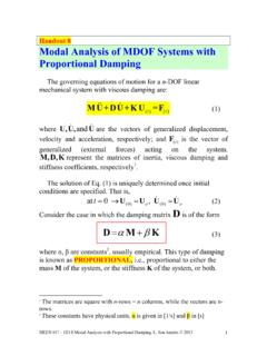
1 MEEN 617 HD#7 undamped Modal Analysis of MDOF Systems . L. San Andr s 2008 1ME617 - Handout 7 ( undamped ) Modal Analysis of MDOF Systems The governing equations of motion for a n-DOF linear mechanical system with viscous damping are: ()()ttMU+DU+KU =F (1) where andU, U,U are the vectors of generalized displacement, velocity and acceleration, respectively; and ()tF is the vector of generalized (external forces) acting on the system. M, D, Krepresent the matrices of inertia, viscous damping and stiffness coefficients, respectively1. The solution of Eq. (1) is uniquely determined once initial conditions are specified. That is, (0)(0)at0,oot= ==UUUU (2) In most cases, conservative Systems , the inertia and stiffness matrices are SYMMETRIC, ,TT==MM KK . The kinetic energy (T) and potential energy (V) in a conservative system are 11,22 TTTV==UMUUKU (3) 1 The matrices are square with n-rows = n columns, while the vectors are n-rows.

2 MEEN 617 HD#7 undamped Modal Analysis of MDOF Systems . L. San Andr s 2008 2In addition, since T > 0, then M is a positive definite matrix2. If V >0, then K is a positive definite matrix. V=0 denotes the existence of a rigid body mode, and makes K a semi-positive matrix. In MDOF Systems , a natural state implies a certain configuration of shape taken by the system during motion. Moreover a MDOF system does not possess only ONE natural state but a finite number of states known as natural modes of vibration. Depending on the initial conditions or external forcing excitation, the system can vibrate in any of these modes or a combination of them. To each mode corresponds a unique frequency knows as a natural frequency. There are as many natural frequencies as natural modes. The modeling of a n-DOF mechanical system leads to a set of n-coupled 2nd order ODEs, Hence the motion in the direction of one DOF, say k, depends on or it is coupled to the motion in the other degrees of freedom, j=1, In the Analysis below, for a proper choice of generalized coordinates, known as principal or natural coordinates, the system of n-ODE describing the system motion is independent of each other, uncoupled.

3 The natural coordinates are linear combinations of the (actual) physical coordinates, and conversely. Hence, the motion in physical coordinates can be construed or interpreted as the superposition or combination of the motions in each natural coordinate. 2 Positive definite means that the determinant of the matrix is greater than zero. More importantly, it also means that all the matrix eigenvalues will be positive. A semi-positive matrix has a zero determinant, with at least an eigenvalues equaling zero. MEEN 617 HD#7 undamped Modal Analysis of MDOF Systems . L. San Andr s 2008 3 For simplicity, begin the Analysis of the system by neglecting damping, D=0. Hence, Eq.(1) reduces to ()()ttMU+KU =F (4) and (0)(0)at0,oot= ==UUUU Presently, set the external force F=0, and let s find the free vibrations response of the system. MU+KU=0 (5) The solution to the homogenous Eq.

4 (5) is simply cos()t U= (6) which denotes a periodic response with a typical frequency . From Eq. (6), 2cos()t U= (7) Note that Eq. (6) is a simplification of the more general solution withand where1stesii == U= (8) Substitution of Eqs. (6) and (7) into the EOM (5) gives: 22cos()cos()cos()ttt MU+KU=0M +K =0M+K =0 and since cos() 0t for most times, then MEEN 617 HD#7 undamped Modal Analysis of MDOF Systems . L. San Andr s 2008 42 M+K =0 (9) or 2 =M K (10) Eq. (10) is usually referred as the standard eigenvalue problem (mathematical jargon): 12where =and ==A MK (11) Eq.(9) is a set of n-homogenous algebraic equations. A nontrivial solution, 0 exists if and only if the determinant of the system of equations is zero, 20 = =M+K (12) Eq. (12) is known as the characteristic equation of the system.

5 It is a polynomial in 2 =, () = = = + +++ = = + (13) This polynomial or characteristic equations has n-roots, the set {}1,2,..kkn =or {}1,2,..kkn = since = . The s are known as the natural frequencies of the system. In the MATH jargon, the s are known as the eigenvalues (of matrix A) MEEN 617 HD#7 undamped Modal Analysis of MDOF Systems . L. San Andr s 2008 5 Knowledge summary a) A n-DOF system has n-natural frequencies. b) If M and K are positive definite, then < . c) If K is semi-positive definite, then = , at least one natural frequency is zero, motion with infinite period. This is known as rigid body mode. Note that each of the natural frequencies satisfies Eq. (9). Hence, associated to each natural frequency (or eigenvalues) there is a corresponding natural mode vector (eigenvector) such that []()1,..,iiin = M+K =0 (14) The n-elements of an eigenvector are real numbers (for undamped system), with all entries defined except for a constant.

6 The eigenvectors are unique in the sense that the ratio between two elements is constant, ()()constant for any ,1,..jikkjin == The actual value of the elements in the vector is entirely arbitrary. Since Eq. (14) is homogenous, if is a solution, so it is for any arbitrary constant . Hence, one can say that the SHAPE of a natural mode is UNIQUE but not its amplitude. For MDOF Systems with a large number of degrees of freedom, n>>3, the eigenvalue problem, Eq. (11), is solved numerically. MEEN 617 HD#7 undamped Modal Analysis of MDOF Systems . L. San Andr s 2008 6 Nowadays, PCs and mathematical computation software allow, with a single (simple) command, the evaluation of all (or some) eigenvalues and its corresponding eigenvectors in real time, even for Systems with thousands of DOFs. Long gone are the days when the graduate student or practicing engineer had to develop his/her own efficient computational routines to calculate eigenvalues.

7 Handout # 9 discusses briefly some of the most popular numerical methods to solve the eigenvalue problem. A this time, however, let s assume the set of eigenpairs {}()1, ,iiin = is known. Properties of natural modes The natural modes (or eigenvectors) satisfy important orthogonality properties. Recall that each eigenpair {}()1, ,iiin = satisfies the equation 2()1,..,iiin = M+K =0. (15) Consider two different modes, say mode-j and mode-k, each satisfying 22()()()()andjjj kkk ==M K M K (16) Pre-multiply the equations above by ()Tk and ()Tj to obtain MEEN 617 HD#7 undamped Modal Analysis of MDOF Systems . L. San Andr s 2008 72()()()()2()()()()andTTjkjkjTTkjkjk == M K M K (17) Now, perform some matrix manipulations. The products TM and TK are scalars, not a matrix nor a vector. The transpose of a scalar is the number itself. Hence, ()()()()()()()()()()()sinceTTTTT jkkjTTkjTTkj=== K K K K K=K and ()()()()()sinceTTTTjkk j= M M M=M for symmetric Systems .

8 Thus, Eqs. (17) are rewritten as 2()()()()2()()()()()and()TTjjkjkTTkjkjka b == M K M K (18) Subtract (b) from (a) above to obtain ()22()()0 Tjk jk = M (19) if jk , for TWO different natural frequencies; then it follows that MEEN 617 HD#7 undamped Modal Analysis of MDOF Systems . L. San Andr s 2008 8for jk ()()0 Tjk= M and ()()0 Tjk= K (20) for jk= ()()TjjjM= M and 2()()TjjjjjKM == K (20) where Kj and Mj are known as the j- Modal stiffness and j- Modal mass, respectively. Define a Modal matrix has as its columns each of the eigenvectors, [] (21) and the Modal properties are written as [][];TTMK== M K (22) where [M] and [K] are diagonal matrices containing the Modal mass and stiffnesses, respectively. The eigenvector set k=1,..n is linearly independent. Hence, any vector (v) in n-dimensional space can be described as a linear combination of the natural modes, ()1njjja=== v a (23) []12112 =+ ++ == v a MEEN 617 HD#7 undamped Modal Analysis of MDOF Systems .

9 L. San Andr s 2008 9 System Response in Modal Coordinates The orthogonality property of the natural modes (eigenvectors) permits the simplification of the Analysis for prediction of system response. Recall that the equations of motion for the undamped system are ()()ttMU+KU =F (4) and (0)0(0)0at0,t= ==UUUU Consider the Modal transformation ()()tt=U q (24)3 And with ()()tt=U q , then EOM (4) becomes: ()tM q+K q=F which offers no advantage in the Analysis . However, premultiply the equation above by T to obtain ()()()TTTt M q+ K q= F (25) and using the properties of the natural modes, [][];TTMK== M K , then Eq. (25) becomes [][]()TtMK=q+q=Q F (26) 3 Eq. (24) sets the physical displacements U as a function of the Modal coordinates q. This transformation merely uses the property of linear independence of the natural modes. MEEN 617 HD#7 undamped Modal Analysis of MDOF Systems .

10 L. San Andr s 2008 10 And since [M] and [K] are diagonal matrices. Eq. (26) is just a set of n-uncoupled ODEs. That is, +=+=+= (27) Or 1, ,jjjKMjjjjjnjnMq Kq Q =+== (28) The set of q s are known as Modal or natural coordinates (canonical or principal, too). The vector ()Tt=Q Fis known as the Modal force vector. Thus, the major advantage of the Modal transformation (24) is that in Modal space the EOMS are uncoupled. Each equation describes a mode as a SDOF system. The unique solution of Eqs. (28) needs of initial conditions specified in Modal space, {},ooqq . Using the Modal transformation, ;oooo==U qU q , it follows 11;ooo o ==q Uq U (28) However, Eq. (28) requires of the inverse of Modal matrix , 1 = I. For Systems with a large number of DOF, n>> 1, finding the matrix 1 is computationally expensive. MEEN 617 HD#7 undamped Modal Analysis of MDOF Systems . L. San Andr s 2008 11A more efficient to determine the initial state {},ooqq in Modal coordinates follows.