Transcription of Microsoft Excel 2016 Advanced - customguide.com
1 Microsoft . Excel 2016 Advanced Quick Reference Card Free Quick References Visit PivotTable Elements PivotTable Layout PivotTable Fields PivotTable Fields Pane Pane The PivotTable Fields pane controls how Active PivotTable Search PivotTable Fields Pane data is represented in the PivotTable. Fields Options Click anywhere in the PivotTable to activate the pane. It includes a Search field, a scrolling list of fields (these are Tools the column headings in the data range Menu used to create the PivotTable), and four areas in which fields are placed. These four areas include: Field List Filters: If a field is placed in the Filters area, a menu appears above the PivotTable.
2 Each unique value from the field is an item in the menu, which can be used to filter PivotTable data. Column Labels: The unique values for the fields placed in the Columns area appear as column headings along the top of the PivotTable. Row Labels: The unique values PivotTable Field for the fields placed in the Rows Areas area appear as row headings along the left side of the PivotTable. PivotTables PivotCharts Values: The values are the meat . Create a PivotTable: Select the data range to Create a PivotChart: Click any cell in a of the PivotTable, or the actual be used by the PivotTable. Click the Insert tab PivotTable and click the Analyze tab on the data that's calculated for the fields on the ribbon and click the PivotTable button ribbon.
3 Click the PivotChart button in the Tools placed in the rows and/or columns in the Tables group. Verify the range and click group. Select a PivotChart type and click OK. area. Values are most often OK. numeric calculations. Modify PivotChart Data: Drag fields into and out Add Multiple PivotTable Fields: Click a field in of the field areas in the task pane. Both the Not all PivotTables will have a field in the field list and drag it to one of the four PivotTable and PivotChart update instantaneously. each area, and sometimes there will be PivotTable areas that contains one or more multiple fields in a single area. fields.
4 Refresh a PivotChart: With the PivotChart selected, click the Analyze tab on the ribbon. The Layout Group Filter PivotTables: Click and drag a field from Click the Refresh button in the Data group. the field list into the Filters area. Click the field's list arrow above the PivotTable and select the Modify PivotChart Elements: With the value(s) you want to filter. PivotChart selected, click the Design tab on the ribbon. Click the Add Chart Element button in Group PivotTable Values: Select a cell in the the Chart Elements group and select the item(s). PivotTable that contains a value you want to you want to add to the chart.
5 Group by. Click the Analyze tab on the ribbon and click the Group Field button. Specify Apply a PivotChart Style: Select the PivotChart Subtotals: Show or hide subtotals and how the PivotTable should be grouped and click and click the Design tab on the ribbon. Select a specify their location in the PivotTable. OK. style from the gallery in the Chart Styles group. Grand Totals: Add or remove grand total Refresh a PivotTable: With the PivotTable Update the Chart Type: With the PivotChart rows for columns and/or rows. selected, click the Analyze tab on the ribbon. selected, click the Design tab on the ribbon. Click Click the Refresh button in the Data group.
6 The Change Chart Type button in the Type Report Layout: Adjust the report layout group. Select a new chart type and click OK. to show in compact, outline, or tabular Format a PivotTable: With the PivotTable form. selected, use the options on the Design tab to Enable PivotChart Drill Down: Click the adjust the PivotTable styles and style options. Analyze tab. Click the Field Buttons list arrow Blank Rows: Emphasize groups of data in the Show/Hide group and select Show by manually adding blank rows between Expand/Collapse Entire Field Buttons. grouped items. Your Organization's Name Here 2018 CustomGuide, Inc. Add your own message, logo, and contact information!
7 To learn more, contact | Macros Troubleshoot Formulas Advanced Formulas Enable the Developer Tab: Click the File tab The Watch Window: Select the cell you want Nested Functions: A nested function is when and select Options. Select Customize to watch. Click the Formulas tab on the one function is tucked inside another function Ribbon at the left. Check the Developer ribbon and click the Watch Window button. as one of its arguments. It looks like this: check box and click OK. Click the Add Watch button. Ensure the correct cell is identified and click Add. =IF(D2>AVERAGE(B2:B10), Yes , No ). Macro Naming Rules: Evaluate a Formula: Select a cell with a Initial Nested Result Result The first character must be a letter.
8 Formula to evaluate. Click the Formulas tab on Function Function If True' If False'. Only letters, numbers, and underscores are the ribbon and click the Evaluate Formula accepted. button. Click the Evaluate button as many The Vlookup Function: The Vlookup function times as required to locate the error. Spaces, periods, and special characters =VLOOKUP(lookup_value, table_array, are not allowed. col_index_num, [range_lookup]) looks for a Advanced Formatting value you specify in the first column of data The name can't exceed 255 characters; it's and then returns a value in the same row from best practice to keep it under 25.
9 Customize Conditional Formatting: Click a column you specify. the Conditional Formatting button on the Record a Macro: Click the Developer tab on Home tab and select New Rule in the menu. the ribbon and click the Record Macro Select a rule type and then edit the styles and button. Type a name, description and specify values. Click OK. where to save it. Click OK. Complete the steps to be recorded. Click the Stop Recording Edit a Conditional Formatting Rule: Click button on the Developer tab. the Conditional Formatting button on the Home tab and select Manage Rules. Select Run a Macro: Click the Developer tab on the the rule you want to edit and click Edit Rule.
10 Ribbon and click the Macros button. Select Make your changes to the rule. Click OK. the macro and click Run. Change the Order of Conditional Logical Functions: Use a logical function Edit a Macro: Click the Developer tab on the Formatting Rules: Click the Conditional such as And, Or, or Not when you want to ribbon and click the Macros button. Select carry out more than one comparison in a Formatting button on the Home tab and a macro and click the Edit button. Make the formula. select Manage Rules. Select the rule you necessary changes to the Visual Basic code want to re-sequence. Click the Move Up or and click the Save button.