Transcription of Mixtures of Normals - Princeton University
1 February 20, 2014 Time: 10 of NormalsIn this chapter, I will review the mixture of Normals modeland discuss various methods for inference with special attentionto Bayesian methods. The focus is entirely on the use of mix-tures of Normals to approximate possibly very high dimensionaldensities. Prior specification and prior sensitivity are importantaspects of Bayesian inference and I will discuss how priorspecification can be important in the mixture of Normals from univariate to high dimensional will be usedto illustrate the flexibility of the mixture of Normals model aswell as the power of the Bayesian approach to inference forthe mixture of Normals model.
2 Comparisons will be made toother density approximation methods such as kernel densitysmoothing which are popular in the econometrics most general case of the mixture of Normals model mixes or averages the normal distribution over a (y| )= (y| , ) ( , | )d d ( )Here ( ) is the mixing distribution . ( ) can be discrete or con-tinuous. In the case of univariate normal Mixtures , an importantexample of a continuous mixture is the scale mixture of (y| )= (y| , ) ( | )d ( )A scale mixture of a normal distribution simply alters the tailbehavior of the distribution while leaving the resultant distribu-tion symmetric.
3 Classic examples include the t distribution and Copyright, Princeton University Press. No part of this book may be distributed, posted, or reproduced in any form by digital or mechanical means without prior written permission of the publisher. February 20, 2014 Time: 10 1double exponential in which the mixing distributions are inversegamma and exponential, respectively (Andrews and Mallows(1974)). For our purposes, we desire a more general form of mix-ing which allows the resultant mixture distribution sufficientflexibility to approximate any continuous distribution to somedesired degree of accuracy.
4 Scale Mixtures do not have sufficientflexibility to capture distributions that depart from normality ex-hibiting multi-modality and skewness. It is also well-known thatmost scale Mixtures that achieve thick tailed distributions suchas the Cauchy or low degree of freedom t distributions also haverather peaked densities around the mode of the distribution . Itis common to find datasets where the tail behavior is thicker thanthe normal but the mass of the distribution is concentrated nearthe mode but with rather broad shoulders ( , Tukey s slash distribution ).
5 Common scale Mixtures cannot exhibit this sortof behavior. Most importantly, the scale mixture ideas do noteasily translate into the multivariate setting in that there arefew distributions on for which analytical results are available(principally the Inverted Wishart distribution ).For these reasons, I will concentrate on finite Mixtures ofnormals. For a finite mixture of Normals , the mixing distributionis a discrete distribution which puts mass on K distinct values of and .p(y| ,{ k, k})= k k (y| k, k)( ) ( ) is the multivariate normal density.
6 (y| , )=(2 ) d/2| | 1/2exp 1/2(y ) 1(y ) ( )dis the dimension of the data, points of thefinite mixture of Normals are often called thecomponentsof themixture. The mixture of Normals model is very attractive fortwo reasons: (1) the model applies equally well to univariate andmultivariate settings; and (2) the mixture of Normals model canachieve great flexibility with only a few components. Copyright, Princeton University Press. No part of this book may be distributed, posted, or reproduced in any form by digital or mechanical means without prior written permission of the publisher.
7 February 20, 2014 Time: 10 of Normals3420 2 2 2 2 of Univariate NormalsFigure illustrates the flexibility of the mixture of normalsmodel for univariate distributions. The upper left corner ofthe figure displays a mixture of a standard normal with anormal with the same mean but 100 times the variance (thered density curve), that is the (0,1)+.05N(0,100).This mixture model is often used in the statistics literature asa model for outlying observations. Mixtures of Normals canalso be used to create a skewed distribution by using a base normal with another normal that is translated to the right or leftdepending on the direction of the desired upper right panel of Figure displays the mix-ture.
8 75N(0,1)+.25N( ,22). This example of constructinga skewed distribution illustrates that Mixtures of Normals donot have to exhibit separation or bimodality. If we positiona number of mixture components close together and assign eachcomponent similar probabilities, then we can create a mixturedistribution with a density that has broad shoulders of the type Copyright, Princeton University Press. No part of this book may be distributed, posted, or reproduced in any form by digital or mechanical means without prior written permission of the publisher.
9 February 20, 2014 Time: 10 1-202468-202468 Figure Mixture of Bivariate Normalsdisplayed in many datasets. The lower left panel of Figure the ( 1,1)+.5N(1,1), a distribution that ismore or less uniform near the mode. Finally, it is obvious that wecan produce multi-modal distributions simply by allocating onecomponent to each desired model. The bottom right panel of thefigure shows the ( 1,.52)+.5N(1,.52). The darkerlines in Figure show a unit normal density for the multivariate case, the possibilities are even broader. Forexample, we could approximate a bivariate density whose con-tours are deformed ellipses by positioning two or more bivariatenormal Mixtures along the principal axis of symmetry.
10 The axis of symmetry can be a curve allowing for the creation of a densitywith banana or any other shaped contour. Figure shows a Copyright, Princeton University Press. No part of this book may be distributed, posted, or reproduced in any form by digital or mechanical means without prior written permission of the publisher. February 20, 2014 Time: 10 of Normals5mixture of three uncorrelated bivariate Normals that have beenpositioned to obtain bent or banana-shaped is an obvious sense in which the mixture of normalsapproach, given enough components, can approximate any mul-tivariate density (see Ghosh and Ramamoorthi (2003) for infinitemixtures and Norets and Pelenis (2011) for finite Mixtures ).