Transcription of mixup: BEYOND EMPIRICAL RISK MINIMIZATION
1 Published as a conference paper at ICLR 2018. mixup: B EYOND E MPIRICAL R ISK M INIMIZATION. Hongyi Zhang Moustapha Cisse, Yann N. Dauphin, David Lopez-Paz . MIT FAIR. A BSTRACT. Large deep neural networks are powerful, but exhibit undesirable behaviors such as memorization and sensitivity to adversarial examples. In this work, we propose [ ] 27 Apr 2018. mixup, a simple learning principle to alleviate these issues. In essence, mixup trains a neural network on convex combinations of pairs of examples and their labels. By doing so, mixup regularizes the neural network to favor simple linear behavior in-between training examples. Our experiments on the ImageNet-2012, CIFAR-10, CIFAR-100, Google commands and UCI datasets show that mixup improves the generalization of state-of-the-art neural network architectures.
2 We also find that mixup reduces the memorization of corrupt labels, increases the robustness to adversarial examples, and stabilizes the training of generative adversarial networks. 1 I NTRODUCTION. Large deep neural networks have enabled breakthroughs in fields such as computer vision (Krizhevsky et al., 2012), speech recognition (Hinton et al., 2012), and reinforcement learning (Silver et al., 2016). In most successful applications, these neural networks share two commonalities. First, they are trained as to minimize their average error over the training data, a learning rule also known as the EMPIRICAL Risk MINIMIZATION (ERM) principle (Vapnik, 1998). Second, the size of these state-of-the- art neural networks scales linearly with the number of training examples. For instance, the network of Springenberg et al.
3 (2015) used 106 parameters to model the 5 104 images in the CIFAR-10 dataset, the network of (Simonyan & Zisserman, 2015) used 108 parameters to model the 106 images in the ImageNet-2012 dataset, and the network of Chelba et al. (2013) used 2 1010 parameters to model the 109 words in the One Billion Word dataset. Strikingly, a classical result in learning theory (Vapnik & Chervonenkis, 1971) tells us that the convergence of ERM is guaranteed as long as the size of the learning machine ( , the neural network) does not increase with the number of training data. Here, the size of a learning machine is measured in terms of its number of parameters or, relatedly, its VC-complexity (Harvey et al., 2017). This contradiction challenges the suitability of ERM to train our current neural network models, as highlighted in recent research.
4 On the one hand, ERM allows large neural networks to memorize (instead of generalize from) the training data even in the presence of strong regularization, or in classification problems where the labels are assigned at random (Zhang et al., 2017). On the other hand, neural networks trained with ERM change their predictions drastically when evaluated on examples just outside the training distribution (Szegedy et al., 2014), also known as adversarial examples. This evidence suggests that ERM is unable to explain or provide generalization on testing distributions that differ only slightly from the training data. However, what is the alternative to ERM? The method of choice to train on similar but different examples to the training data is known as data augmentation (Simard et al.)
5 , 1998), formalized by the Vicinal Risk MINIMIZATION (VRM) principle (Chapelle et al., 2000). In VRM, human knowledge is required to describe a vicinity or neighborhood around each example in the training data. Then, additional virtual examples can be drawn from the vicinity distribution of the training examples to enlarge the support of the training distribution. For instance, when performing image classification, it is common to define the vicinity of one image as the set of its horizontal reflections, slight rotations, and mild scalings. While data augmentation consistently leads to improved generalization (Simard et al., 1998), the procedure is dataset-dependent, and thus requires the use of expert knowledge. Furthermore, data augmentation assumes that the . Alphabetical order.
6 1. Published as a conference paper at ICLR 2018. examples in the vicinity share the same class, and does not model the vicinity relation across examples of different classes. Contribution Motivated by these issues, we introduce a simple and data-agnostic data augmenta- tion routine, termed mixup (Section 2). In a nutshell, mixup constructs virtual training examples x = xi + (1 )xj , where xi , xj are raw input vectors y = yi + (1 )yj , where yi , yj are one-hot label encodings (xi , yi ) and (xj , yj ) are two examples drawn at random from our training data, and [0, 1]. Therefore, mixup extends the training distribution by incorporating the prior knowledge that linear interpolations of feature vectors should lead to linear interpolations of the associated targets. mixup can be implemented in a few lines of code, and introduces minimal computation overhead.
7 Despite its simplicity, mixup allows a new state-of-the-art performance in the CIFAR-10, CIFAR- 100, and ImageNet-2012 image classification datasets (Sections and ). Furthermore, mixup increases the robustness of neural networks when learning from corrupt labels (Section ), or facing adversarial examples (Section ). Finally, mixup improves generalization on speech (Sections ). and tabular (Section ) data, and can be used to stabilize the training of GANs (Section ). The source-code necessary to replicate our CIFAR-10 experiments is available at: To understand the effects of various design choices in mixup, we conduct a thorough set of ablation study experiments (Section ). The results suggest that mixup performs significantly better than related methods in previous work, and each of the design choices contributes to the final performance.
8 We conclude by exploring the connections to prior work (Section 4), as well as offering some points for discussion (Section 5). 2 F ROM E MPIRICAL R ISK M INIMIZATION TO mixup In supervised learning, we are interested in finding a function f F that describes the relationship between a random feature vector X and a random target vector Y , which follow the joint distribution P (X, Y ). To this end, we first define a loss function ` that penalizes the differences between predictions f (x) and actual targets y, for examples (x, y) P . Then, we minimize the average of the loss function ` over the data distribution P , also known as the expected risk: Z. R(f ) = `(f (x), y)dP (x, y). Unfortunately, the distribution P is unknown in most practical situations. Instead, we usually have access to a set of training data D = {(xi , yi )}ni=1 , where (xi , yi ) P for all i = 1.
9 , n. Using the training data D, we may approximate P by the EMPIRICAL distribution n 1X. P (x, y) = (x = xi , y = yi ), n i=1. where (x = xi , y = yi ) is a Dirac mass centered at (xi , yi ). Using the EMPIRICAL distribution P , we can now approximate the expected risk by the EMPIRICAL risk: Z n 1X. R (f ) = `(f (x), y)dP (x, y) = `(f (xi ), yi ). (1). n i=1. Learning the function f by minimizing (1) is known as the EMPIRICAL Risk MINIMIZATION (ERM). principle (Vapnik, 1998). While efficient to compute, the EMPIRICAL risk (1) monitors the behaviour of f only at a finite set of n examples. When considering functions with a number parameters comparable to n (such as large neural networks), one trivial way to minimize (1) is to memorize the training data (Zhang et al., 2017). Memorization, in turn, leads to the undesirable behaviour of f outside the training data (Szegedy et al.)
10 , 2014). 2. Published as a conference paper at ICLR 2018. # y1, y2 should be one-hot vectors ERM mixup for (x1, y1), (x2, y2) in zip(loader1, loader2): lam = (alpha, alpha). x = Variable(lam * x1 + (1. - lam) * x2). y = Variable(lam * y1 + (1. - lam) * y2). (). loss(net(x), y).backward(). (b) Effect of mixup ( = 1) on a () toy problem. Green: Class 0. Or- ange: Class 1. Blue shading indicates (a) One epoch of mixup training in PyTorch. p(y = 1|x). Figure 1: Illustration of mixup, which converges to ERM as 0. However, the na ve estimate P is one out of many possible choices to approximate the true distribu- tion P . For instance, in the Vicinal Risk MINIMIZATION (VRM) principle (Chapelle et al., 2000), the distribution P is approximated by n 1X. P (x , y ) = (x , y |xi , yi ), n i=1.
![arXiv:0706.3639v1 [cs.AI] 25 Jun 2007](/cache/preview/4/1/3/9/3/1/4/b/thumb-4139314b93ef86b7b4c2d05ebcc88e46.jpg)
![arXiv:1301.3781v3 [cs.CL] 7 Sep 2013](/cache/preview/4/d/5/0/4/3/4/0/thumb-4d504340120163c0bdf3f4678d8d217f.jpg)
![@google.com arXiv:1609.03499v2 [cs.SD] 19 Sep 2016](/cache/preview/c/3/4/9/4/6/9/b/thumb-c349469b499107d21e221f2ac908f8b2.jpg)