Transcription of Molecular dynamics simulation
1 Molecular dynamics simulationCS/CME/BioE/Biophys/BMI 279 Oct. 5, 2021 Ron Dror1 Outline Molecular dynamics (MD): The basic idea Equations of motion Key properties of MD simulations Sample applications Limitations of MD simulations Software packages and force fields Accelerating MD simulations Monte Carlo simulation2 Molecular dynamics : The basic idea3 The idea Mimic what atoms do in real life, assuming a given potential energy function The energy function allows us to calculate the force experienced by any atom given the positions of the other atoms Newton s laws tell us how those forces will affect the motions of the atoms4 Energy (U)PositionPositionBasic algorithm Divide time into discrete time steps, no more than a few femtoseconds (10 15 s) each At each time step: Compute the forces acting on each atom, using a Molecular mechanics force field Move the atoms a little bit.
2 Update position and velocity of each atom using Newton s laws of motion5 Molecular dynamics movieEquations of motion7 Specifying atom positions For a system with N atoms, we can specify the position of all atoms by a single vector x of length 3N This vector contains the x, y, and z coordinates of every atomx=x1y1z1x2y2z2 xNyNzNSpecifying forces A single vector F specifies the force acting on every atom in the system For a system with N atoms, F is a vector of length 3N This vector lists the force on each atom in the x-, y-, and z- directions Notation: Force on atom 1 in the x-direction: Potential energy: U(x) How quickly potential energy changes as one moves atom 1 in the x-direction: F=F1,xF1,yF1,zF2,xF2,yF2,z FN,xFN,yFN,z= U(x)= U x1 U y1 U z1 U x2 U y2 U z2 U xN U yN U zNF1,x U x1 Equations of motion Newton s second law: F = ma where F is force on an atom, m is mass of the atom, and a is the atom s acceleration Recall that: where x represents coordinates of all atoms, and U is the potential energy function Velocity is the derivative of position, and acceleration is the derivative of velocity We can thus write the equations of motion as.
3 10F(x)= U(x)dxdt=vdvdt=Fx()mSolving the equations of motion This is a system of ordinary differential equations For N atoms, we have 3N position coordinates and 3N velocity coordinates Analytical (algebraic) solution is impossible Numerical solution is straightforward where t is the time step11dxdt=vdvdt=Fx()mvi+1=vi+ tF(xi)mxi+1=xi+ tvivi+1=vi+ tF(xi)mxi+1=xi+ tviSolving the equations of motion Straightforward numerical solution: In practice, people use time symmetric integration methods such as Leapfrog Verlet This gives more accuracy You re not responsible for this12vi+12=vi 12+ tF(xi)mxi+1=xi+ tvi+12vi+1=vi+ tF(xi)mxi+1=xi+ tvivi+1=vi+ tF(xi)mxi+1=xi+ tvivi+12=vi 12+ tF(xi)mxi+1=xi+ tvi+12 Key properties of MD simulations13 Atoms never stop jiggling In real life, and in an MD simulation , atoms are in constant motion.
4 They will not simply go to an energy minimum and stay there Given enough time, the simulation samples the Boltzmann distribution That is, the probability of observing a particular arrangement of atoms is a function of the potential energy In reality, one often does not simulate long enough to reach all energetically favorable arrangements This is not the only way to explore the energy surface ( , sample the Boltzmann distribution), but it s a pretty effective way to do so14 Energy (U)PositionPositionEnergy conservation Total energy (potential + kinetic) should be conserved In atomic arrangements with lower potential energy, atoms move faster In practice, total energy tends to grow slowly with time due to numerical errors (rounding errors) In many simulations, one adds a mechanism to keep the temperature roughly constant (a thermostat )15 Water is important Ignoring the solvent (the molecules surrounding the molecule of interest) leads to major artifacts Surrounding molecules include.
5 Water, salt ions ( , sodium, chloride), lipids of the cell membrane Two options for taking solvent into account Explicitly represent solvent molecules High computational expense but more accurate Usually assume periodic boundary conditions (a water molecule that goes off the left side of the simulation box will come back in the right side, like in PacMan) Implicit solvent Mathematical model to approximate average effects of solvent Less accurate but faster 16 Explicit solventWater (and ions)ProteinCell membrane (lipids)Sample applications18 Determining where drug molecules bind, and how they exert their effectsWe used simulations to determine where this molecule binds to its receptor, and how it changes the binding strength of molecules that bind elsewhere (in part by changing the protein s structure).
6 We then used that information to alter the molecule such that it has a different et al., Nature 2013 Determining functional mechanisms of proteinsSimulation started from active structure vs. Inactive structureRosenbaum et al., Nature 2010; Dror et al., PNAS 2011 We performed simulations in which an adrenaline receptor transitions spontaneously from its active structure to its inactive structure We used these to describe the mechanism by which drugs binding to one end of the receptor cause the other end of the receptor to change shape (activate)Understanding the process of protein folding For example, in what order do secondary structure elements form?
7 But note that MD is generally not the best way to predict the folded structureLindorff-Larsen et al., Science 2011 Increasingly, MD is used together with experimental approaches to address more complicated problems Example: Suomivuori, Latorraca, .., Dror, Science, 2020 Molecular mechanism of biased signaling in a prototypical G protein coupled receptor Collaboration with Lefkowitz lab (Duke), Kruse lab (Harvard)Source: HPCWireNote: The most challenging part of many MD studies is analyzing the data that the simulations produceMD simulation isn t just for proteins Simulations of other types of molecules are common All of the biomolecules discussed in this class Materials science simulations23 Limitations of MD simulations24 Timescales Simulations require short time steps for numerical stability 1 time step 2 fs (2 10 15 s) Structural changes in proteins can take nanoseconds (10 9 s), microseconds (10 6 s), milliseconds (10 3 s)
8 , or longer Millions to trillions of sequential time steps for nanosecond to millisecond events (and even more for slower ones) Until recently, simulations of 1 microsecond were rare Advances in computer power have enabled microsecond simulations, but simulation timescales remain a challenge Enabling longer-timescale simulations is an active research area, involving: Algorithmic improvements Parallel computing Hardware: GPUs, specialized hardware 25 Force field accuracy Molecular mechanics force fields are inherently approximations They have improved substantially over the last decade, but many limitations remain In practice, one needs some experience to know what to trust in a simulation26 Here force fields with lower scores are better, as assessed by agreement between simulations and experimental data.
9 Even the force fields with scores of zero are imperfect, however! Lindorff-Larsen et al., PLOS One, 2012 Covalent bonds cannot break or form during standard MD simulations Once a protein is created, most of its covalent bonds do not break or form during typical function. A few covalent bonds do form and break more frequently (in real life): Disulfide bonds between cysteines Acidic or basic amino acid residues can lose or gain a hydrogen ( , a proton) Various more advanced techniques do allow simulations to capture breaking or formation of at least some covalent bonds27 Software packages and force fields (These topics are not required material for this class, but they ll be useful if you want to do MD simulations) 28 Software packages Multiple Molecular dynamics software packages are available.
10 Their core functionality is similar GROMACS, AMBER, NAMD, Desmond, OpenMM, CHARMM Dominant package for visualizing results of simulations: VMD ( Visual Molecular dynamics )29 Force fields for Molecular dynamics Most MD simulations today use force fields from one of three families: CHARMM, AMBER, OPLS-AA Multiple versions of each Do not confuse CHARMM and AMBER force fields with CHARMM and AMBER software packages They all use strikingly similar functional forms Common heritage: Lifson s Consistent force field from mid-20th-century Some emerging force fields use neural networks fit to results of quantum chemistry calculations30 Accelerating MD simulations 31 Why is MD so computationally intensive?