Multinomial Logistic Regression Models with SAS …

1 1 PharmaSUG 2017 - Paper HA02 Multinomial Logistic Regression Models with SAS PROC SURVEYLOGISTIC Marina Komaroff, Noven Pharmaceuticals, New York, NY ABSTRACT Proportional odds Logistic regressions are popular Models to analyze data from the complex population survey design that includes strata, clusters, and weights. However, when the proportional odds assumption is violated (p-value < .05 for chi-square statistic), the use of Multinomial Logistic Regression Models for survey designs becomes challenging. This paper provides guidance in using Multinomial Logistic Regression Models to estimate and correctly interpret the relationships between predictor and multiple levels of nominal outcome with and without interaction term. The author developed a SAS MACRO utilizing PROC SYRVEYLOGISTIC that will help researchers to conduct statistical analyses. The National Health and Nutrition Examination Survey (NHANES) is a probability sample of the US population.

2 These data sets were used in the examples of Multinomial Logistic Regression modeling techniques. Statistical analysis was conducted using the SAS System for Windows (release ; SAS Institute Inc., Cary, ) The author is convinced that this paper will be useful to SAS-friendly researchers who analyze the complex population survey data with Multinomial Logistic Regression Models . INTRODUCTION Multinomial Logistic regressions model log odds of the nominal outcome variable as a linear combination of the predictors. A multivariate method for Multinomial outcome variable compares one for each pair of outcomes. For example, if the outcome variable has three categories then two Models are tested with Multinomial Regression comparing simultaneously the second and third level versus the first (reference). The ratio of the probability of one outcome category over the probability of the reference category is often referred to as relative risk or odds, and Regression coefficients are relative risk ratios or odds ratios for a unit change in the predictor variable.

3 The complexity increases when Multinomial Models are applied to data from population survey designs. The recent updates in PROC SURVEYLOGISTIC made the use of Multinomial Logistic regressions more inviting, but left users with challenging interpretations of the results. This paper concentrates on use and interpretation of the results from Multinomial Logistic Regression Models utilizing PROC SURVEYLOGISTIC. The user-friendly SAS MACRO written by the author can easily be applied for analysis of different research questions. DESCRIPTION DATABASE Eight cross-sectional (NHANES 2-year cycles) data sets were concatenated to examine relationships between predictor and Multinomial outcome. Eight time points (NHANES cycles from 1999-2000 through 2013-2014) were used to determine if the relationships (odds ratios) have changed over 16-year time period. METHOD The analysis was conducted by Multinomial Logistic Regression Models across all surveys that accommodated the complex multistage sample survey design utilizing appropriate sampling weights following NHANES Analytic and Reporting guidance.

4 [1,2] The Models utilized the NOMCAR option in PROC SURVEYLOGISTIC to treat missing values in the variance computation as not missing completely at random for Taylor series variance estimation. Multinomial Logistic Regression Models , continued 2 In the Models , a set of k levels of outcome variable are modeled as generalized logits that contrast each level with the reference: GLogiti { Pr [Outcome i] } = Log {Pr[Outcome i] / Pr[Outcome j] }, for Outcome i=1, 2, ..,k where j=1, 2,.., k-1, j < i estimating probability of each level versus the reference ( 2 vs. 1 , 3 vs. 1 , etc. if 1-ref.). For the predictor variable (for example, gender), the coefficient gender = Log (odds ratio) = Log {oddsfemale / oddsmale}= Log[oddsfemale] Log[oddsmale]. This odds ratio estimates the relationship between predictor and outcome. Particularly, the odds ratio for gender estimates the ratio between odds of advanced versus early level of outcome (for example, 3 vs. 1 ) for females and the same odds for males.

5 The interaction term between predictor and time (eight NHANES cycles) can be tested. A significant interaction indicates that the relationship (odds ratio) between predictor and outcome has changed over time. In the model without interaction term, the Odds Ratio (OR) greater than 1 indicates that probability of advance versus earlier level of outcome (reference) is higher among females versus males keeping the covariates at the constant level. With the interaction term, the Logit equals to gender + gender*time, where gender*time is the coefficient of the interaction. In other words, with increase of one unit of time (NHANES cycle), the Log (OR) is adding the value of Time* gender*time; which is the same as OR changing exponentially by multiplying exp( gender) to the (exp( gender*time))time, where time = 1, 2,..8. If gender*time is close to zero which is the same as exp( gender*time) is close to one, then no significant change in the relationship is observed over the years.

6 APPLICATION Objectives The objective was to estimate the association between Gender (female vs. male) and BMI categories (normal, overweight, and obese), and how the associations have changed from 1999 to 2014 for the US American adults (18 years or older). Outcome Variable - Three levels of BMI: normal (<25 kg/m2), overweight ( 25 - < 30 kg/m2), and obese ( 30 kg/m2). Predictor Variable - Gender: Females versus Males (ref.). Covariates Age, and Race groups (NHANES[2]: 1='Non-Hispanic White', 2 = 'Non-Hispanic Black', 3 = 'Mexican American', 4 = 'Other'). EXAMPLE No 1: Evaluate the association between Gender and BMI categories and examine if the associations have changed from 1999 to 2014. EXAMPLE No 2: Evaluate the association between Gender and BMI categories and examine if the associations have changed from 1999 to 2014 adjusting for Age and Race. MACRO TO PERFORM Multinomial Logistic Regression Models Parameters for Multinomial Logistic Regression Model %MNLRM( sds=A, /* The name of SAS data set */ inp=gender, /* Predictor Variable */ refinp=%str(Male) , /* Reference group for Predictor */ outp=BMIGRP, /* Outcome Variable */ cov=%str(race), /* Covariates: names of the variables */ domain=sel, /* Domain used for selected population */ domainx=%str( ), /* Population from Domain to exclude */ num=1 ); /* Model Number */ %MACRO MNLRM(sds= A, inp=gender, refinp=%str(Male), outp=BMIGRP, cov=%str(), domain=sel, domainx=%str( ), num=1 ); Multinomial Logistic Regression Models , continued 3 *RUN MODEL **; proc surveylogistic data=&SDS NOMCAR; format cycle cyclef.

7 Age agef. gender genderf. race racef.; /* prepare for possible covariates */ strata sdmvstra; cluster sdmvpsu; class &inp(ref="&refinp") &cov/param=glm ; domain model &outp(descending) = &inp|cycle &cov /link=glogit expb ; weight mec16yr; /* recalculate weight to combine surveys */ %DO i=1 %To 8; lsmeans &inp /at cycle=&i e ilink oddsratio cl diff; %END; ods output lsmeans=LSM&num Diffs=D&num Type3=T3A&num ParameterEstimates = PE&num DomainSummary=DS store Model run; quit; Title "Table: Odds Ratios "; proc sort data=D&num out=D1&num(keep=effect cycle probZ &outp DOMAIN OddsRatio LOWEROR UPPEROR); by domain &outp cycle ; where (domain ne "&domainx"); run; *PUT ODDS RATIOS FROM EACH TIME POINT INTO THE ONE LAST RECORD **; data D2&num(rename=(effect=variable)); set D1 by domain &outp cycle; format response $1.; retain OR1-OR8 LowerOR1-LowerOR8 UpperOR1-UpperOR8 .; response=put(&outp, 1.)

8 ; if then do; %DO j=1 %TO 8; OR UpperOR LowerOR %END; end; %DO cycle=1 %TO 8; if cycle=&cycle then do; OR&cycle=OddsRatio; UpperOR&cycle=UpperOR; LowerOR&cycle=LowerOR; end; %END; if then output; run; *GENERATE OUTPUT **; filename outf&num "C:\&study\out\& "; ODS RTF file=outf title "Output 1: Type 3 Analysis of Effects"; proc print data=T3A where domain ne " run; title "Parameter Estimates"; proc print data=PE where (domain ne "&domainx") and (ClassVal0 ne " run; title "Output 2: Odds Ratios with 95% Confidence Intervals (CI)"; proc print data=D2 by domain ; var variable &outp OR1-OR8 LowerOR1- LowerOR8 UpperOR1-UpperOR8 ; run; Multinomial Logistic Regression Models , continued 4 ** FOREST PLOTS **; data DD set D reference=1; col1=1; response= ef1=put(cycle, cyclef.); ef2=put(cycle, cyclef.); if (domain ne "&domainx") and (response > reference) and (oddsratio ne .); label col1="Reference " response=" run; ODS graphics on; proc sort data=DD by domain response cycle; run; title "Output 3: Forest Plots"; proc sgplot data=DD&num UNIFORM=all ; by domain response ; format response respf.)

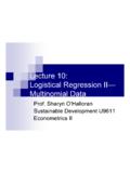
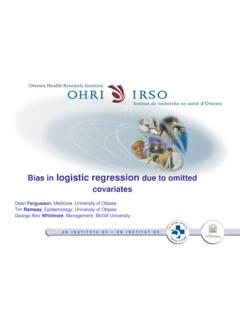
9 ; keylegend /title=""; scatter x=oddsratio y=ef1 / xerrorlower=lowerOR xerrorupper=upperOR markerattrs=(symbol=DiamondFilled size=8); refline 1 / NAME= "BMI" axis=x; xaxis label="OR and 95% CI " min=0; yaxis label="Female vs. Male "; run; * Regression **; proc sort data=LSM&num out=LSM where domain ne ""; by domain run; title "Output 4: Analysis of Covariates" ; proc GLM data=LSM by domain format &inp & cycle cyclef.; class &inp (ref=" model estimate= cycle|&inp /solution; output out=r&num p=pred&num L95=lower&num U95=upper run; quit; ODS graphics off; ODS RTF close; %MEND; EXAMPLE No 1 %MNLRM(sds=a4, inp=gender, refinp=%str(Male) , outp=BMIGRP, cov=%str(), domain=sel, domainx=%str( ), num=1 ) Multinomial Logistic Regression Models , continued 5 Output 1: Type 3 Analysis of Effects Variable DF WaldChiSq P-value Gender 2 <.0001 NHANES cycle 2 <.0001 NHANES cycle*Gender 2 Output 2: Odds Ratios with 95% Confidence Intervals (CI) for Females compared to Males* BMI Group 1999-2000 OR (95% CI) 2001-2002 OR (95% CI) 2003-2004 OR (95% CI) 2005-2006 OR (95% CI) 2007-2008 OR (95% CI) 2009-2010 OR (95% CI) 2011-2012 OR (95% CI) 2013-2014 OR (95% CI) p-value A.)

10 Overweight vs Normal ( ) ( ) ( ) ( ) ( ) ( ) ( ) ( ) B. Obese vs Normal ( ) ( ) ( ) ( ) ( ) ( ) ( ) ( ) *Significant associations are presented in bold Output 3: Forest Plots A. BMI Groups: Overweight versus Normal B. BMI Groups: Obese versus Normal Output 4: Analysis of Covariates A. BMI Groups: Overweight versus Normal B. BMI Groups: Obese versus Normal Multinomial Logistic Regression Models , continued 6 CONCLUSIONS FOR EXAMPLE #1: 1. Type 3 analysis of effects demonstrated that gender and time are significant predictors (p < .05) for BMI. The interaction term was not significant (p > .05) indicating these relationships have not changed over time. (Output 1) 2. The chance of being in overweight vs normal BMI category is significantly lower for Females compared to Males across all years from 1999 through 2014, but the relationships (odds ratios) have not changed over time.