Transcription of Simple Logistic Regression.notes - mc.vanderbilt.edu
1 1 III. INTRODUCTION TO Logistic REGRESSION1. Simple Logistic Regressiona) Example: APACHE II Score and Mortality in SepsisThe following figure shows 30 day mortality in a sample of septic patients as a function of their baseline APACHE II Score. Patients are coded as 1 or 0 depending on whether they are dead or alive in 30 days, II Score at BaselineDiedSurvived30 Day Mortality in Patients with SepsisWe wish to predict death from baseline APACHE II score in these (x) be the probability that a patient with score xwill that linear regression would not work well here since it could produce probabilities less than zero or greater than II Score at BaselineDiedSurvived30 Day Mortality in Patients with Sepsis2b) Sigmoidal family of Logistic regression curvesLogistic regressionfits probability functions of the following form:pab ab() exp()/( exp())xxx=+ ++1 This equation describes a family of sigmoidal curves, three examples of which are given below.
2 ()ab+ x0x - p()/()x +=010 0 For negative values of x, exp asand (x)c) Parameter values and the shape of the regression curvepab ab() exp()/(exp())xxx=+ ++1 For now assume that > very large values of x, and henceexp()ab+ xp()()x + = (x)pab ab() exp()/(exp())xxx=+ ++1xx=-+ =ab a b/,0p().x=+=11 1 05bgWhen and henceThe slope of (x) when (x)=.5 is controls how fast (x) rises from 0 to given , controls were the 50% survival point is located. Data with a lengthy transition from survival to death should have a low value of . 010510152025303540xDiedSurvivedWe wish to choose the best curve to fit the that has a sharp survival cut off point between patients who live or die should have a large value of .4pab ab() exp()/(exp())xxx=+ ++11-=p()xd) The probability of death under the Logistic modelThis probability is{ }Hence probability of survival =++-+++11exp() exp()exp()abababxxxlog( ( ) (( ))ppabxx x1-=+The log odds of death equals{ }, and the odds of death ispp ab( ) (( )) exp()xxx1-= +=+ +11(exp())abxe) The logit functionFor any number between 0 and 1 the logit function is defined bylogit() log( /())ppp=-1 Let di=xibe the APACHE II score of theithpatient10:: patient dies patient livesththiiRST() () Pr[ 1]ii iEdxd=p ==Then the expected value of diis Thus we can rewrite thelogistic regression equation{ } as{ }logit( ( ))( )iiiEdxx=p =a+b52.
3 Contrast Between Logistic and Linear RegressionIn linear regression , the expected value ofyigiven xiisforEyxii()=+abin=12, ,..,ab+xiis the linear is the random component of the model, which has a normal a normal distribution with standard deviation .In Logistic regression , the expected value of given xiis E(di) = idlogit(E(di)) = + xi for i= 1, 2, .. , n[]iixp=pidis dichotomous with probability of event []iixp=pit is the random component of the modellogit is the link function that relates the expected value of the random component to the linear Maximum Likelihood EstimationIn linear regression we used the method of least squares to estimate regression coefficients. In generalized linear models we use another approach called maximum likelihood estimation. The maximum likelihood estimate of a parameter is that value that maximizes the probability of the observed estimate and by those values and that maximize the probability of the observed data under the Logistic regression model.
4 A b6 Bas e line APACHE II ScoreNu mb e r of PatientsNu mb e r of De ath sBas eline APACHE II S c o reNu mb e r of Patie ntsNu mb e r of De ath s010 20136210 21179341 2214124 11 0 23 13 7593 241186 14 3 25 12 87124 26628225 27759333 283110 19 6 29 7 411 31 5 30 5 412 17 5 31 3 313 32 13 32 3 314 25 7 33 1 115 18 7 34 1 116 24 8 35 1 117 27 8 36 1 118 19 13 37 1 119 15 7 41 1 0 This data is analyzed as tabulate fateDeath by 30 |days | Freq. Percent +-----------------------------------aliv e | 279 | 175 +-----------------------------------Tota l | 454 histogram apache [fweight=freq ], discrete(start=0, width=1) Score at Baseline.
5 Scatter proportion of Deaths with Indicated Score010203040 APACHE Score at Baseline8 Logit estimates Number of obs = 454LR chi2(1) = > chi2 = likelihood = Pseudo R2 = | Coef. Std. Err. z P>|z| [95% Conf. Interval]-------------+----------------- ---------------------------------------- -------apache | .1156272 .0159997 .0842684 .146986_cons| .2765283 a b= .1156272= ab() exp()/( exp())xxx=+ ++1exp( + .1156272 )1 exp( + .1156272 )xx=+()exp( + .1156272 20) exp( + .1156272 20) p==+ logit( ( ))( )iiiEdxx=p =a+ of Death by 30 days010203040 APACHE Score at BaselineProportion of Deaths with Indicated ScorePr(fate)94. Odds Ratios and the Logistic regression Modela) Odds ratio associated with a unit increase in xThe log odds that patients with APACHE II scores of xand x+ 1 will die arelogit{ }(())pabxx=+(())()pababbxxx+=+ +=++11andlogit{ } { } from { } gives(())(())ppxx+-1logit = logitlog())()log()()ppppxxxx+-+FHGIKJ--F HGIKJ111 1=and henceexp( ) is the odds ratio for death associated with a unit increase in x.
6 ( ())( ( ))ppxx+-1logit = logitpppp()/(())()/(())xxxx+-+-FHGIKJ111 1= logA property of Logistic regression is that this ratio remains constant for all values of x. 105. 95% Confidence Intervals for Odds Ratio EstimatesIn our sepsis example the parameter estimate for apache( ) was .1156272 with a standard error of .0159997. Therefore, the odds ratio for death associated with a unit rise in APACHE II score is exp(.1156272) = a 95% confidence interval of (exp( - ), exp( + )) = ( , ).6. Quality of Model fitIf our model is correct then() logit observed proportionix=a+bIt can be helpful to plot the observed log odds against ixa+b11-2-10123 Log odds of Death in 30 days010203040 APACHE Score at Baselineobs_logoddsLinear predictionThen it can be shown that the standard error of is= sex a+b 222 2xxaabbs+ s + s7. 95% Confidence Interval forLet and denote the variance of and.
7 Let denote the covariance between and .[]xp2 as2 bs a b abs a bxa+b sexx a+b a+b A 95% confidence interval for is 12-4-2024010203040 APACHE Score at Baselinelb_logodds/ub_logoddsobs_logodds Linear predictionHence, a 95% confidence interval for is , whereand[]xp[][]() ,LUxxpp[] se a+b - a+b p= +a+b- a+b [] se 1 seUxxxxx a+b + a+b p= +a+b+ a+b A 95% confidence interval for is xa+b sexx a+b a+b ()()()()exp/ 1 expiiixxxp = a+b+ a+ Score at Baselinelb_prob/ub_probProportion Dead by 30 DaysPr(fate)It is common to recode continuous variables into categorical variables in order to calculate odds ratios for, say the highest quartile compared to the centile apache, centile(25 50 75)-- Binom. Interp.
8 --Variable | Obs Percentile Centile [95% Conf. Interval]-------------+----------------- ---------------------------------------- ----apache | 454 25 10 9 11| 50 14 15| 75 20 19 21. generate float upper_q= apache >= 20. tabulate upper_qupper_q | Freq. Percent +-----------------------------------0 | 334 | 120 +-----------------------------------Tota l | 454 cc fate upper_q if apache >= 20 | apache <= 10 Proportion| Exposed Unexposed | Total Exposed-----------------+--------------- ---------+----------------------Cases | 77 25 | 102 | 43 101 | 144 +------------------------+-------------- --------Total | 120 126 | 246 | || Point estimate | [95% Conf.]
9 Interval]|------------------------+----- -----------------Odds ratio | | (exact)Attr. frac. ex. | .8617719 | .7451951 .9256007 (exact)Attr. frac. pop | .6505533 |+-------------------------------------- ---------chi2(1) = Pr>chi2 = approach discards potentially valuable information and may notbe as clinically relevant as an odds ratio at two specific we can calculate the odds ratio for death for patients at the 75thpercentile of Apache scores compared to patients at the 25thpercentile ( (20))20p=a+b logit( (10))10p=a+b logitSubtracting gives ()()()() ()()20 / 120log10 10 / 110 p-p=b = = p-p Hence, the odds ratio equals exp( ) = problem with this estimate is that it is strongly dependent on the accuracy of the Logistic regression , the odds ratio equals exp( ) = problem with this estimate is that it is strongly dependent on the accuracy of the Logistic regression Stata we can calculate the 95% confidence interval for this oddsratio as follows.
10 Lincom 10*apache, eform( 1) 10 apache = 0--------------------------------------- ---------------------------------------f ate | exp(b) Std. Err. z P>|z| [95% Conf. Interval]-------------+----------------- ---------------------------------------- -------(1) | .5084803 Logistic regression generalizes to allow multiple covariateslogit1221( ( ))..iiikikEdxxx=a+b +b + +bwherexi1, x12, .., xikare covariates from the ithpatient and 1, .. k, are known parametersdi=1:ithpatient suffers event of interest0:otherwise Multiple Logistic regression can be used for many purposes. Oneof these is to weaken the logit-linear assumption of Simple Logistic regression using restricted cubic Restricted Cubic Splines1t2t3t12,, ,kttt"Linear before and after . 1tktPiecewise cubic polynomials between adjacent knots( of the form ) 32axbxcx d+++These curves have kknots located at.