Neural Ordinary Differential Equations

1 Neural Ordinary Differential Equations Ricky T. Q. Chen*, Yulia Rubanova*, Jesse Bettencourt*, David Duvenaud University of Toronto, Vector Institute {rtqichen, rubanova, jessebett, [ ] 15 Jan 2019. Abstract We introduce a new family of deep Neural network models. Instead of specifying a discrete sequence of hidden layers, we parameterize the derivative of the hidden state using a Neural network. The output of the network is computed using a black- box Differential equation solver. These continuous-depth models have constant memory cost, adapt their evaluation strategy to each input, and can explicitly trade numerical precision for speed. We demonstrate these properties in continuous-depth residual networks and continuous-time latent variable models. We also construct continuous normalizing flows, a generative model that can train by maximum likelihood, without partitioning or ordering the data dimensions.}

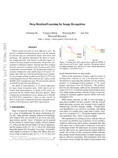
2 For training, we show how to scalably backpropagate through any ODE solver, without access to its internal operations. This allows end-to-end training of ODEs within larger models. 1 Introduction Residual Network ODE Network 5 5. Models such as residual networks, recurrent Neural network decoders, and normalizing flows build com- 4 4. plicated transformations by composing a sequence of transformations to a hidden state: 3 3. Depth Depth ht+1 = ht + f (ht , t ) (1) 2 2. D. where t {0 .. T } and ht R . These iterative 1 1. updates can be seen as an Euler discretization of a continuous transformation (Lu et al., 2017; Haber 0 5 0 5 0 5 0 5. and Ruthotto, 2017; Ruthotto and Haber, 2018). Input/Hidden/Output Input/Hidden/Output What happens as we add more layers and take smaller Figure 1: Left: A Residual network defines a steps?

3 In the limit, we parameterize the continuous discrete sequence of finite transformations. dynamics of hidden units using an Ordinary differen- Right: A ODE network defines a vector tial equation (ODE) specified by a Neural network: field, which continuously transforms the state. dh(t) Both: Circles represent evaluation locations. = f (h(t), t, ) (2). dt Starting from the input layer h(0), we can define the output layer h(T ) to be the solution to this ODE initial value problem at some time T . This value can be computed by a black-box Differential equation solver, which evaluates the hidden unit dynamics f wherever necessary to determine the solution with the desired accuracy. Figure 1 contrasts these two approaches. Defining and evaluating models using ODE solvers has several benefits: Memory efficiency In Section 2, we show how to compute gradients of a scalar-valued loss with respect to all inputs of any ODE solver, without backpropagating through the operations of the solver.

4 Not storing any intermediate quantities of the forward pass allows us to train our models with constant memory cost as a function of depth, a major bottleneck of training deep models. 32nd Conference on Neural Information Processing Systems (NeurIPS 2018), Montr al, Canada. Adaptive computation Euler's method is perhaps the simplest method for solving ODEs. There have since been more than 120 years of development of efficient and accurate ODE solvers (Runge, 1895; Kutta, 1901; Hairer et al., 1987). Modern ODE solvers provide guarantees about the growth of approximation error, monitor the level of error, and adapt their evaluation strategy on the fly to achieve the requested level of accuracy. This allows the cost of evaluating a model to scale with problem complexity. After training, accuracy can be reduced for real-time or low-power applications.

5 Parameter efficiency When the hidden unit dynamics are parameterized as a continuous function of time, the parameters of nearby layers are automatically tied together. In Section 3, we show that this reduces the number of parameters required on a supervised learning task. Scalable and invertible normalizing flows An unexpected side-benefit of continuous transforma- tions is that the change of variables formula becomes easier to compute. In Section 4, we derive this result and use it to construct a new class of invertible density models that avoids the single-unit bottleneck of normalizing flows, and can be trained directly by maximum likelihood. Continuous time-series models Unlike recurrent Neural networks, which require discretizing observation and emission intervals, continuously-defined dynamics can naturally incorporate data which arrives at arbitrary times.

6 In Section 5, we construct and demonstrate such a model . 2 Reverse-mode automatic differentiation of ODE solutions The main technical difficulty in training continuous-depth networks is performing reverse-mode differentiation (also known as backpropagation) through the ODE solver. Differentiating through the operations of the forward pass is straightforward, but incurs a high memory cost and introduces additional numerical error. We treat the ODE solver as a black box, and compute gradients using the adjoint sensitivity method (Pontryagin et al., 1962). This approach computes gradients by solving a second, aug- mented ODE backwards in time, and is applicable to all ODE solvers. This approach scales linearly with problem size, has low memory cost, and explicitly controls numerical error.

7 Consider optimizing a scalar-valued loss function L(), whose input is the result of an ODE solver: Z t1 . L(z(t1 )) = L z(t0 ) + f (z(t), t, )dt = L (ODES olve(z(t0 ), f, t0 , t1 , )) (3). t0. To optimize L, we require gradients with respect to . The first step is to determining how the gradient of the loss depends on the hidden state z(t) at each instant. This quantity is called the adjoint a(t) = L/ z(t). Its dynamics are given by another ODE, which can be thought of as the State instantaneous analog of the chain rule: Adjoint State da(t) f (z(t), t, ). = a(t)T (4). dt z We can compute L/ z(t0 ) by another call to an ODE solver. This solver must run backwards, starting from the initial value of L/ z(t1 ). One complication is that solving this ODE requires Figure 2: Reverse-mode differentiation of an ODE the knowing value of z(t) along its entire tra- solution.

8 The adjoint sensitivity method solves jectory. However, we can simply recompute an augmented ODE backwards in time. The aug- z(t) backwards in time together with the adjoint, mented system contains both the original state and starting from its final value z(t1 ). the sensitivity of the loss with respect to the state. Computing the gradients with respect to the pa- If the loss depends directly on the state at multi- rameters requires evaluating a third integral, ple observation times, the adjoint state must be which depends on both z(t) and a(t): updated in the direction of the partial derivative of Z t0. dL f (z(t), t, ). the loss with respect to each observation. = a(t)T dt (5). d t1 . 2. The vector-Jacobian products a(t)T f T f z and a(t) in (4) and (5) can be efficiently evaluated by automatic differentiation, at a time cost similar to that of evaluating f.

9 All integrals for solving z, a and L. can be computed in a single call to an ODE solver, which concatenates the original state, the adjoint, and the other partial derivatives into a single vector. Algorithm 1 shows how to construct the necessary dynamics, and call an ODE solver to compute all gradients at once. Algorithm 1 Reverse-mode derivative of an ODE initial value problem Input: dynamics parameters , start time t0 , stop time t1 , final state z(t1 ), loss gradient L/ z(t1 ). L. s0 = [z(t1 ), z(t 1). , 0| | ] . Define initial augmented state def aug_dynamics([z(t), a(t), ], t, ): . Define dynamics on augmented state return [f (z(t), t, ), a(t)T f T f z , a(t) ] . Compute vector-Jacobian products L L. [z(t0 ), z(t 0). , ] = ODES olve(s0 , aug_dynamics, t1 , t0 , ) . Solve reverse-time ODE.

10 L L. return z(t0 ) , . Return gradients Most ODE solvers have the option to output the state z(t) at multiple times. When the loss depends on these intermediate states, the reverse-mode derivative must be broken into a sequence of separate solves, one between each consecutive pair of output times (Figure 2). At each observation, the adjoint must be adjusted in the direction of the corresponding partial derivative L/ z(ti ). The results above extend those of Stapor et al. (2018, section ). An extended version of Algorithm 1 including derivatives t0 and t1 can be found in Appendix C. Detailed derivations are provided in Appendix B. Appendix D provides Python code which computes all derivatives for by extending the autograd automatic differentiation package. This code also supports all higher-order derivatives.