Transcription of Notes on the Euler Equations
1 Notes on the Euler EquationsThese Notes describe how to do a piecewise linear or piecewise parabolic method for the Euler Euler equation propertiesThe Euler Equations in one dimension appear as: t+ ( u) x=0(1) ( u) t+ ( uu+p) x=0(2) ( E) t+ ( uE+up) x=0(3)These represent conservation of mass, momentum, and is the density,uis the one-dimensional velocity,pis the pressure, andEis the total energy / mass, and can be expressed in terms ofthe specific internal energy and kinetic energies as:E=e+12u2(4)The Equations are closed with the addition of an equation of state :p= e( 1)(5)where is the ratio of specific heats for the gas/fluid (for an ideal , monatomic gas, =5/3).In this form, the Equations are said to be inconservative form.
2 They can be written as:Ut+[F(U)]x=0(6)withU= u E F(U) = u uu+p uE+up (7)An alternate way to express these Equations is using theprimitive variables: ,u, 1: Show that the Euler Equations in primitive form can be written asqt+A(q)qx=0(8)whereq= up A(q) = u 00u1/ 0 p u (9)The eigenvalues ofAcan be found via|A I|=0, where|..|indicates the determinant and are 2: Show that the eigenvalues of A are ( )=u c, ( )=u, (+)=u+c where the speedof sound is c=p p/ .M. Zingale Notes on the Euler equations1(April 16, 2013)We ll use the symbols{ , ,+}to denote the eigenvalues and their corresponding eigenvectors though-out these Notes . These eigenvalues are the speeds at which information propagates for the fluid the eigenvalues are real, this system (the Euler Equations ) is said to behyperbolic.
3 Additionally, sinceA=A(q), the system is said to bequasi-linear. The right and left eigenvectors can be found via:A r( )= ( )r( );l( )A= ( )l( )(10)where ={ , ,+}corresponding to the three waves, and there is one right and one left eigenvector foreach of the 3: Show that the right eigenvectors are:r( )= 1 c/ c2 r( )= 100 r(+)= 1c/ c2 (11)and the left eigenvectors are:l( )= 0 2c12c2 l( )= 1 0 1c2 l(+)= 0 2c12c2 (12)Note that in general, there can be an arbitrary constant in front of each eigenvector. Here they arenormalized such that l(i) r(j)= final form of the Equations is called thecharacteristic form. Here, we wish to diagonalize the take the matrixRto be the matrix of right eigenvectors,R= (r( )|r( )|r(+)), andLis the correspondingmatrix of left eigenvectors.
4 Note thatL R=I=R L, andL=R 4: Show that =LAR is a diagonal matrix with the diagonal elements simply the 3 eigen-values we found , we can write our system as:wt+ wx=0(13)Here, theware the characteristic variables. Note that we cannot in general integratedw=Ldqto writedown the characteristic quantities. Since is diagonal, this system is a set of decoupled advection-likeequations. If the system were linear, then the solution to each would simply be to advect the quantityw( )at the wave speed ( ).The way to think about this system is that there are 3 wave speeds (one for each eigenvalue) and eachwave carries with it a change in the characteristic variable. Sincedq=L 1dw=Rdw, the jump in theprimitive variable across each wave is proportion to the right-eigenvector associated with that wave.
5 So,for example, sincer( )is only non-zero for the density element, this then means that only density jumpsacross the ( )=uwave pressure and velocity are constant across this wave (see for example, Toro [12],Ch. 2, 3 or LeVeque [7] for a thorough discussion). Figure 1 shows the three waves emanating from aninitial Reconstruction of interface statesWe will solve the Euler Equations using a high-orderGodunov method a finite volume method wherebythe fluxes through the interfaces are computed by solving the Riemann problem for our system. Thefinite-volume update for our system appears as:Un+1i=Uni+ t x Fn+1/2i 1/2 Fn+1/2i+1/2 (14)M. Zingale Notes on the Euler equations2(April 16, 2013) 1 0 1densityx 0 1 0 1velocityx 1 0 1pressurexFigure 1: Evolution following from an initial discontinuity atx= These particular conditions arecalled theSod problem, and in general, a setup with two states separated by a discontinuity is calleda shock-tube problem.
6 Here we see the three waves propagating away from the initial left (u c) wave is a rarefaction, the middle (u) is the contact discontinuity, and the right (u+c)is a shock. Note that all 3 primitive variables jump across the left and right waves, but only thedensity jumps across the middle wave. This reflects the right Zingale Notes on the Euler equations3(April 16, 2013)ii+1i+1/2Un+1/2i+1/2,LUiUn+1/2i+1/2 ,RUi+1F(Un+1/2i+1/2)Figure 2: The left and right states at interfacei+1/2. The arrow indicates the flux through theinterface, as computed by the Riemann solver using these states as says that each of the conserved quantities inUchange only due to the flux of that quantity throughthe boundary of the of approximating the flux itself on the interface, we find an approximation to the state on theinterface,Un+1/2i 1/2andUn+1/2i+1/2and use this with the flux function to define the flux through the interface:Fn+1/2i 1/2=F(Un+1/2i 1/2)(15)Fn+1/2i+1/2=F(Un+1/2i+1/2)(16)To find this interface state, we predict left and right statesat each interface (centered in time), which arethe input to the Riemann solver.
7 The Riemann solver will then look at the characteristic wave structureand determine the fluid state on the interface, which is then used to compute the flux. This is illustratedin Figure 2. The fluxes allow us to update the state in time as:Un+1i=Uni+ t x Fn+1/2i 1/2 Fn+1/2i+1/2 (17)Finally, although we use the conserved variables for the final update, in constructing the interfacestates it is often easier to work with the primitive variables. These have a simpler characteristic interface states in terms of the primitive variables can be converted into the interface states of theconserved variables through a simple algebraic these interface states requires reconstructing the cell-average data with a piecewise con-stant, linear, or parabolic polynomial and doing characteristic tracing to see how much of each charac-teristic quantity comes to the interface over t/2.
8 Since we are comfortable working with the primitivevariables, the reconstruction is done on those, and they arethen projected into the characteristic variables(using the left- and right-eigenvectors) to determine how much of each characteristic quantity is carriedby each of the 3 waves. We look at several methods Piecewise constantThe simplest possible reconstruction of the data is piecewise constant. This is what was done in theoriginal Godunov method. For the interface marked byi+1/2, the left and right states on the interfaceare simply:Ui+1/2,L=Ui(18)Ui+1/2,R=Ui+1(19)T his does not take into account in any way how the stateUmay be changing through the cell. As aresult, it is first-order accurate in space, and since no attempt was made to center it in time, it is first-orderaccurate in Zingale Notes on the Euler equations4(April 16, 2013)ii 1i+1i 2i+2 Figure 3: Piecewise linear reconstruction of the cell averages.
9 The dotted line shows the unlimitedcenter-difference slopes and the solid line shows the limited Piecewise linearFor higher-order reconstruction, we first convert from the conserved variables,U, to the primitive vari-ables,q. These have a simpler characteristic structure, making themeasier to work with. Here we con-sider piecewise linear reconstruction the cell average data is approximated by a line with non-zero slopewithin each cell. Figure 3 shows the piecewise linear reconstruction of some constructing the left state at the interfacei+1/2 (see Figure 2). Just like for the advectionequation, we do a Taylor expansion through x/2 to bring us to the interface, and t/2 to bring us to themidpoint in time. Starting withqi, the cell-centered primitive variable, expanding to the right interface(to create the left state there) gives:qn+1/2i+1/2,L=qni+ x2 q x i+ t2 q t i|{z}= A q/ x+.
10 (20)=qni+ x2 q x i t2 A q x i(21)=qni+12 1 t xAi qi(22)where qiis the reconstructed slope of the primitive variable in thatcell (similar to how we compute itfor the advection equation). We note that the terms truncated in the first line areO( x2)andO( t2), soour method will be second-order accurate in space and with the advection equation, we limit the slope such that nonew minima or maxima are intro-duced. Any of the slope limiters used for linear advection apply here as well. We represent the limitedslope as can decomposeA qin terms of the left and right eigenvectors and sum over all the waves thatmovetowardthe interface. First, we recognize thatA=R Land recognizing that the 1 in Eq. 22 is theidentity,I=LR, we rewrite this expression as:qn+1/2i+1/2,L=qni+12 RL t xR L i qi(23)We see the common factor ofL q.