Numerical Solution of Differential Equations

1 Numerical Solution of Differential EquationsLiz BradleyDepartment of Computer ScienceUniversity of ColoradoBoulder, Colorado, USA 80309-0430c 1998 Revised versionc 2002, Report on Curricula and Teaching CT003-981 ordinary Differential EquationsA differential equation expresses a set of constraints amongthe derivatives of an unknown function. Here s asimple example:ddtx(t) =ax(t)(1)What this means is that the derivative of the unknown function is equal toatimes the unknown function compactness, the independent variable (t, here) is often omitted and the notationdxdtis often abbreviatedwith a dot, like so: xor with a prime, like so:x . Using these two notations, equation (1) becomes x=axorx =ax, solve a differential equation, you (generally) can t justintegrate both sides. Rather, you have to findsome function that satisfies the constraints expressed in that equation in the example above, some functionx(t) whose derivativex (t) is equal to a constant multiple of the function itself1.

2 There is no general, foolproofway to do this unless the equation is very simple. Differential Equations textbooks are cookbooks that giveyou lots of suggestions about approaches, but there are lotsof differential Equations (DEs) that simply don thaveanalytic solutions that is, solutions that you can write down. These Equations can only be solvednumerically, using the kinds of methods that are described in these Equations are interesting and useful to scientists and engineers because they model thephysical world: that is, they capture the physics of a system, and their solutions emulate the behavior of thatsystem. The class of differential Equations that have no analytic solutions has a highly specific and interestinganalog in the physical world: they model so-calledchaoticsystems. This means that Numerical methods forsolving ODEs are an essential tool for anyone (like me) who studies equation (ODE) has only one independent variable, and all derivatives in it aretaken with respect to that variable.

3 Most often, this variable is timet, but some books usexas the independentvariable; pay careful attention to what the derivative is taken with respect to so you don t get s an example of where ODEs come from. Consider a massmon a spring with spring constantk:1 The answer isx(t) =beat+c, wherea, bandcare you definexas the position of the end of the spring, as shown in the figure,and setx= 0 at the point wherethe end of the spring would naturally rest if it were unloaded( , ifm= 0), you can write the following forcebalance at the mass: F=mamg kx=ma(2)Accelerationais the second derivative of position:a=x , so the equation becomes:mg kx=mx Themgforce is gravity;kxis Hooke s law for the force exerted by a spring. The signs ofmgandkxareopposite because gravity pulls in the direction of positivexand the spring pulls in the direction of negativex. Gathering terms and dividing through bymgives you the following ODE for the spring-mass system:x (t) +kmx(t) g= 0 Note that this ODE model does not include the effects of friction; if friction plays an important role in thesystem, this model is independent variabletonly appearsimplicitlyin this equation that is, hidden in the time dependenceof the functionx(t).

4 This means that thephysics(the governing Equations ) of the system is not a functionof time. If, on the other hand, someone were holding the top ofthe spring and moving it up and down in asinusoidal pattern, the apparent gravity acting on the masswould change sinusoidally (much as the gravitychanges in an elevator that is starting or stopping), and theequation would look like this:x (t) +kmx(t) g0sint= 0 The variabletappearsexplicitlyin this ODE by itself, and not wrapped in the brackets of a function likex(t). Systems where this occurs are an ODE is the degree of the highest derivative in that =axis a first-orderODE,x tanx = 2 is a third-order ODE, and the spring-mass equation above is second order. Annth-order ODE can be transformed intonfirst-order ODEs (annth-order ODE system ), and vice versa2. Thistransformation requires the introduction of helper variables. I ll illustrate with the third-order (n= 3)examplex 1(t) + 36 logx 1(t) x21(t) + sin 2t= 141.

5 The first step is to rewrite the ODE with the highest-order term by itself on the left-hand side:x 1= 14 +x21 36 logx 1 sin 2t2 This means that the order of an ODE system is equal to the number of first-order ODEs in the corresponding ODE The second step is to definen 1 helper variables, like so:x 1=x2, x 2=x33. The third step is to rewrite the equation from step 1 using the helper variables, with no derivative signsat all on the right-hand side and only one on the left-hand side:x 3= 14 +x21 36 logx2 sin 2t4. Finally, one appends the Equations that define the helper variables to that rewritten equation, obtainingthenth-order system:x 1=x2x 2=x3x 3= 14 +x21 36 logx2 sin 2tThis set of first-order ODEs is equivalent tox 1= 14 +x21 36 logx 1 sin 2t, as you can see by substitutingthe first two Equations into the third. The variables that appear on the left-hand side of an ODE system aretermed thestate variablesof the system.

6 Thestate vector~xof this system is (x1x2x3)Tand the ODE systemis of the form~x =~f(~x, t)I will use this standard form throughout these notes. For autonomous systems,~fdoesn t actually depend ontat all, so the standard form collapses to~x =~f(~x)Here s a famous third-order ODE system, derived by Edward Lorenz, that models the physics of a fluidthat is being heated from below:~x =~f(~x) = x y z = a(y x)rx y xzxy bz (3)This system of ODEs is autonomous (no explicitts on the right-hand side). It is alsononlinear, as you cansee by looking at equation (3) above; if any of right-hand sides of any of these Equations contain any termsthat are nonlinear ( , products, transcendentals, powers, ..) in the state variables, then the whole systemis nonlinear. Here, the product termsxzandxyare the culprits;a, r, andbare constants. The simpleexamplex =ax, in contrast, islinear;x 1+ 36 logx 1 x21+ sin 2t= 14 is nonlinear because of the log andx21terms.

7 This terminology can be a little confusing; the individual Equations in the system (3) like thex =a(y x) one may look linear by themselves, but you need to rememberthat the whole thing is apackage: asingle(albeit vector-valued) function of a vector-valued argument. You might also think that thederivative operator makes the Equations nonlinear, but it doesn t work that way. Thesolutionsto the ODEare another matter: an ODE that is linear in its dependent variables can have solutions that are nonlinear inits independent variable ( ,x =axand its solutionx(t) =eat).The order of the ODE affects the width of the Solution . The Solution to the first-order ODEx =ax,for example, is the single functionx(t) =beat. The Solution to annth-order ODE system is a set ofnfunctions, each of which both obeys the rules of the ODE and describes the evolution of one state variable:x1(t), x2(t), x3(t) in thex 1+ 36 logx 1 x21+ sin 2t= 14 example3, orx(t), y(t),andz(t) for the Lorenzsystem.

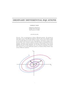
8 Thesenfunctions define a trajectory in thestate spaceof that system: the space whose axes are thestate variables. One can plot the three pieces of the ODE Solution individually, against time, or against oneanother, as shown in figure speaking, in a nonautonomous system like this, onemust considertto be another state variable, but this won t be afactor in our study of these kinds of 1: The Lorenz system. From top to bottom:x(t) versust,y(t) versust,z(t) versust, andz(t) versusx(t). A 3D plot of all three pieces of the Solution against one another withx(t) on thexaxis,y(t) on theyaxis, andz(t) on thezaxis is called (t0,x0)t0tx0tx (t0,x0,v0)tyy0x0t0xv (t0,x0,v0)(a)(b)Figure 2: (a) A Solution to a first-order ODE (b) A Solution to asecond-order ODE. Solid lines show thestate-space trajectories and dashed lines show the derivative vectors at example state-space points (x0,t0)in part (a) and (x0,y0,t0) in part (b).

9 2 Numerical Solution of Single-Step MethodsSolving an ODE numerically means computing thetrajectory~x(t) from some initial condition~x(t0). This isdifferent from the general, analytic Solution , which tells you~x(t)everywhere. A useful metaphor for ODEsolvers is to think of figuring out where a ball will roll on a landscape, given the slope of the landscape andthe initial position of the ball. An ODE is a machine that takes a point and gives you the slope at that point,and an ODE solver is a Numerical method that uses these slopesto compute the trajectory from some initialcondition. A first-order ODE describes the slope of a 2D landscape ( , for instance); see figure 2(a). Asecond-order ODE describes the slope of a 3D landscape, as shown in figure 2(b). Note that the slope vectorin this image in Figure 2 has two pieces: anx-direction slope and ay-direction slope. The ball rolling on thatlandscape reacts tobothof rest of this section describes four basic Numerical ODE Solution algorithms: Forward Euler, BackwardEuler, Trapezoidal, and fourth-order Runge-Kutta.

10 All four of these methods take an ODE in the standardform~x =~f(~x, t), an initial condition~x(t0), and a step sizeh, and generate an approximation of the Solution ~x(t) fort > t0. There arelotsof other Numerical ODE solvers; this is only a small sample. There are differentnames for these methods, by the way; many people call Backward Euler Modified Euler or Implicit Euler. Forward EulerForward Euler (FE) is the simplest and most obvious Numerical ODE solver. It uses the slope at each point,computed using the ODE, to extrapolate and find the next point:~xn+1=~xn+h~x nNote that~x is a derivative, so its units are in distance per time. Multiplying it byh an increment oftime puts theh~x nterm in units of :solve the first-order ODE systemx (t) = 2x(t) +tfromx(0) = 1 for two steps using ForwardEuler with a time steph= step:x( ) =x(0) +h(x (0))= 1 + ( )( 2(1) + 0)= step:x( ) =x( ) +h(x ( ))= + ( )( 2( ) + )= :solve the Lorenz system on page 3 of these notes witha= 16,r= 50, andb= 4 from the initialcondition [x, y, z] = [0,1,2] for one step using Forward Euler with a time steph= arithmetic here is identical to that in the first-order system above, except that all thexs are nowthree-vectors instead of scalars: xyz t= xyz t=0+h x y z t=0 xyz t= 012 + 16(1 0)50(0) 1 (0)(2)(0)(1) (4)(2) xyz t= 012 +.