Transcription of Ordinal logistic regression (Cumulative logit modeling ...
1 Categorical outcome variables (Beyond 0/1 data) (Chapter 6) Ordinal logistic regression (Cumulative logit modeling ) Proportion odds assumption Multinomial logistic regression Independence of irrelevant alternatives, Discrete choice models Although there are some differences in terms of interpretation of parameter estimates, the essential ideas are similar to binomial logistic regression . Ordered categorical outcomes Examples: tumor stage (local, regional, distant), disability severity (none, mild, moderate severe), Likert items (strong disagree, disagree, agree, strongly agree), weight status (underweight, normal, overweight, obese) Dichotomize at some fixed level corresponding to a logical outcome of interest, maybe it is particularly of interest to distinguish between tumors detected at the regional stage and those at the distant stage, hence we could dichotomize the stages at that point.
2 Could treat the ordered categories as a continuous variable. If it is reasonable to assume that a unit difference between one level and the next is constant, then this can be a reasonable approach. Often Likert items are simply treated as if they are continuous scores with unit increments 1,2,3,4. Both above methods are suboptimal since they either throw out information (dichotomizing) or make uncheckable assumptions (treating as continuous) A popular way to model the ordered categories directly is using an ordered logistic regression , also called Ordinal or cumulative logistic regression and also called a proportional odds model which aptly states the model s main assumption Ordered logistic regression Let Yi take on categories 1, 2.
3 , K, the ordered logistic regression model is ~ Multinomial ( 1, 2,.., ) +1+..+ 1+..+ = > = 0 + , =1,.., 1 and 01 02 .. 0 Note that P(Y j) = 1 + 2 + .. + j . Hence we are modeling the log odds of being greater than the cutoff value j as compared to being less than it and a similar expression applies for j at all K 1 levels. For example, if K = 4 then we are modeling the odds of: 2,3,4 vs. 1; and 3,4 vs. 1,2; and 4 vs. 1,2,3. Note that the intercept parameter 0j is different for each j allowing the jump in probability from one level to the next to differ, but that the relating the predictor X to the logit of the outcome is constant across all j.
4 This constant - interpreted as the log odds ratio of being at a higher level compared to a lower level associated with a unit increase in X - is a strong assumption and is referred to as the proportional odds assumption and can be tested. Assessing the proportional odds assumption The ordered logistic regression model basically assumes that the way X is related to being at a higher level compared to lower level of the outcome is the same across all levels of the outcome. The global test for proportional odds considers a model > = 0 + , =1.
5 , 1 and tests whether 1 = 2 = .. = K 1 for all p elements of hence it is a test with p (K 2) degrees of freedom. This test is known to be problematic since it is anti-conservative (rejects more than it should) plus as a global test it does not tell us where the problem of non-proportionality is or how practically important it is. Bender R and Grouven U (1998) Using Binary logistic regression Models for Ordinal Data with Non-proportional Odds, J Clin Epidemiology, 51(10) 809-816. recommends fitting separate tests for each covariate (from unadjusted models) recommends comparing slopes from separately fit logistic regression models discusses PPOM - partially proportional odds model and generalized logit models Proportional odds modeling in SAS, stata , and R In SAS: PROC logistic works, by default if there are more than 2 categories it will perform Ordinal logistic regression with the proportional odds assumption.
6 By default SAS will perform a Score Test for the Proportional Odds Assumption . Can also use Proc GENMOD with dist=multinomial link=cumlogit in stata : Estimate the Ordinal logistic regression model using ologit and then to check proportional odds use the post-estimation command . brant, detail Download the add-on file . net from jslsoc/ stata / The available packages will be listed with the package names shown in blue. Click on the blue name of the package you want to install ( spost9ado) and follow the instructions. In R: can use the lrm() function in the Design (now rms) Package; can also be fit using polr() in the MASS Package; and the vglm() function in the VGAM Package; and Example: Birthweight example: stata Mother s baseline bmi category is regressed on age and parity.
7 Xi: ologit c_baseline_bmi age_lmp ~t _Iparityftp_0-2 (naturally coded; _Iparityftp_0 omitted) Ordered logistic regression Number of obs = 2000 LR chi2(3) = Prob > chi2 = Log likelihood = Pseudo R2 = ---------------------------------------- ---------------------------------------- c_baseline_bmi | Coef. Std. Err. z P>|z| [95% Conf.]
8 Interval] ---------------+------------------------ ---------------------------------------- _Iparityftp_1 | .1536237 .0992048 .3480616 _Iparityftp_2 | .663759 .1073115 .4534323 .8740857 age_lmp | .0227954 .0080193 .0070779 .0385129 ---------------+------------------------ ---------------------------------------- /cut1 | .2307082 /cut2 | .2248569 .6102129 /cut3 | .2265837.
9 Ologit, or <-- to show odds ratios .. Birthweight example: stata (test for proportional odds) . brant, detail Estimated coefficients from j-1 binary regressions y>1 y>2 y>3 _Iparityftp_1 .15520257 .28841532 _Iparityftp_2 .245485 .70531414 .75288058 age_lmp .07588288 .01187854 .01914656 _cons .37355111 Brant Test of Parallel regression Assumption Variable | chi2 p>chi2 df -------------+-------------------------- All | 6 -------------+-------------------------- _Iparityft~1 | 2 _Iparityft~2 | 2 age_lmp | 2 ---------------------------------------- A significant test statistic provides evidence that the parallel regression assumption has been violated.
10 Note: -brant- is not fully compatible with newer version of stata . Have to use -xi- prefix for categorical variables. Birthweight example: SAS (1) Data Set Response Variable c_baseline_bmi Number of Response Levels 4 Model cumulative logit Optimization Technique Fisher's scoring Number of Observations Read 2000 Number of Observations Used 2000 Response Profile Ordered c_baseline_ Total Value bmi Frequency 1 4 582 2 3 311 3 2 945 4 1


