Transcription of Part 1 Examples of optimization problems
1 49 Wolfgang BangerthPart 1 Examples of optimization problems50 Wolfgang BangerthLet X be a Banach space; let f : X R {+ } g: X Rne h: X Rnibe functions on X, find x X so thatQuestions: Under what conditions on X, f, g, h can we guarantee that (i) there is a solution; (ii) the solution is unique; (iii) the solution is speaking: f(x) min!g(x) = 0h(x) 0 What is an optimization problem?51 Wolfgang BangerthWhat is an optimization problem? x={u,y} is a set of design and auxiliary variables thatcompletely describe a physical, chemical, economical model; f(x) is an objective function with which we measure howgood a design is; g(x) describes relationships that have to be met exactly(for example the relationship between y and u) h(x) describes conditions that must not be exceededThen find me that x for whichQuestion: How do I find this x?
2 In practice: f(x) min!g(x) = 0h(x) 052 Wolfgang BangerthWhat is an optimization problem? optimization problems are often subdivided into classes:Linear vs. Nonlinear Convex vs. NonconvexUnconstrained vs. Constrained Smooth vs. NonsmoothWith derivatives vs. Derivativefree Continuous vs. Discrete Algebraic vs. ODE/PDE Depending on which class an actual problem falls into, there are different classes of Wolfgang BangerthExamplesLinear and nonlinear functions f(x) on a domain bounded by linear inequalities54 Wolfgang BangerthExamplesStrictly convex, convex, and nonconvex functions f(x)55 Wolfgang BangerthAnother non-convex function with many (local) may want to find the one global Wolfgang BangerthOptima in the presence of (nonsmooth)
3 Wolfgang BangerthSmooth and non-smooth nonlinear Wolfgang BangerthMathematical description:x={u,y}:u are the design parameters ( the shape of the car)y is the flow field around the carf(x):the drag force that results from the flow fieldg(x)=y-q(u)=0:constraints that come from the fact that there is a flowfield y=q(u) for each design. y may, for example, satisfythe Navier-Stokes equationsApplications: The drag coefficient of a car59 Wolfgang BangerthInequality constraints:(expected sales price profit margin) - cost(u) 0volume(u) volume(me, my wife, and her bags) 0material stiffness * safety factor- max(forces exerted by y on the frame) 0legal margins(u) 0 Applications: The drag coefficient of a car60 Wolfgang BangerthAnalysis:linearity.
4 F(x) may be linearg(x) is certainly nonlinear (Navier-Stokes equations)h(x) may be nonlinearconvexity: ??constrained: yessmooth:f(x) yesg(x) yesh(x) some yes, some noderivatives: available, but probably hard to compute in practicecontinuous:yes, not discreteODE/PDE:yes, not just algebraicApplications: The drag coefficient of a car61 Wolfgang BangerthRemark:In the formulation as shown, the objective function was of the formf(x) = cd(y)In practice, one often is willing to trade efficiency for cost, we are willing to accept a slightly higher drag coefficient if the cost is smaller.
5 This leads to objective functions of the formf(x) = cd(y) + a cost(u)orf(x) = cd(y) + a[cost(u)]2 Applications: The drag coefficient of a car62 Wolfgang BangerthApplications: Optimal oil production strategiesPermeability fieldMathematical description:x={u,y}:u are the pumping rates at injection/production wellsy is the flow field (pressures/velocities)f(x):the cost of production and injection minus sales price ofoil integrated over lifetime ofreservoir (or -NPV)g(x)=y-q(u)=0:constraints that come from the fact that there is a flowfield y=q(u) for each u.
6 Y may, for example, satisfythe multiphase porous media flow equationsOil saturation63 Wolfgang BangerthApplications: Optimal oil production strategiesInequality constraints h(x) 0:Uimax-ui 0(for all wells i):Pumps have a maximal pumping rate/pressureproduced_oil(T)/available_o il(0) c 0:Legislative requirement to produce at least a certain fractionc - water_cut(t) 0 (for all times t):It is inefficient to produce too much waterpressure d 0 (for all times and locations):Keeps the reservoir from collapsing64 Wolfgang BangerthApplications: Optimal oil production strategiesAnalysis:linearity:f(x) is nonlinearg(x) is certainly nonlinearh(x) may be nonlinearconvexity: noconstrained: yessmooth:f(x) yesg(x) yesh(x) yesderivatives: available, but probably hard to compute in practicecontinuous:yes, not discreteODE/PDE:yes, not just algebraic65 Wolfgang BangerthApplications: Switching lights at an intersectionMathematical description:x={T, ti1, ti2}.
7 Round-trip time T for the stop light system, switch-green and switch-red times for all lights if(x):number of cars that can pass the intersection perhour; Note: unknown as a function, but we can measure it66 Wolfgang BangerthApplications: Switching lights at an intersectionInequality constraints h(x) 0:300 T 0:No more than 5 minutes of round-trip time, so that peopledon't have to wait for too longt2i-t1i 5 0 (for all lights i):At least 5 seconds of green for everyonet1(i+1)-t2i 5 0:At least 5 seconds of all-red between different greens67 Wolfgang BangerthApplications: Switching lights at an intersectionAnalysis:linearity:f(x) ?
8 ?h(x) is linearconvexity: ??constrained: yessmooth:f(x) ??h(x) yesderivatives: not availablecontinuous:yes, not discreteODE/PDE:no68 Wolfgang BangerthApplications: Trajectory planningMathematical description:x={y(t),u(t)}:position of spacecraft and thrust vector at time tminimize fuel consumptionNewton's lawDo not get too close to the sunOnly limited thrust availablem y t u t =0f x = 0T u t dt y t d0 0umax u t 069 Wolfgang BangerthApplications: Trajectory planningAnalysis:linearity:f(x) is nonlinearg(x) is linearh(x) is nonlinearconvexity: noconstrained: yessmooth.
9 Yes, herederivatives: computablecontinuous:yes, not discreteODE/PDE:yesNote: Trajectory planning problems are often called optimal Wolfgang BangerthApplications: Data fitting 1 Mathematical description:x={a,b}:parameters for the model f(x)=1/N i |yi-y(ti)|2:mean square difference between predicted valueand actual measurementy t =1alogcosh abt 71 Wolfgang BangerthApplications: Data fitting 1 Analysis:linearity:f(x) is nonlinearconvexity: ?? (probably yes)constrained: nosmooth:yesderivatives: available, and easy to compute in practicecontinuous:yes, not discreteODE/PDE:no, algebraic72 Wolfgang BangerthApplications: Data fitting 2 Mathematical description:x={a,b}:parameters for the model f(x)=1/N i |yi-y(ti)|2:mean square difference betweenpredicted value and actual measurementy t =at b73 Wolfgang BangerthApplications: Data fitting 2 Analysis:linearity:f(x) is quadraticConvexity: yesconstrained: nosmooth:yesderivatives.
10 Available, and easy to compute in practicecontinuous:yes, not discreteODE/PDE:no, algebraicNote: Quadratic optimization problems (even with linear constraints) are easy to solve!74 Wolfgang BangerthApplications: Data fitting 3 Mathematical description:x={a,b}:parameters for the model f(x)=1/N i |yi-y(ti)|:mean absolute difference between predictedvalue and actual measurementy t =at b75 Wolfgang BangerthApplications: Data fitting 3 Analysis:linearity:f(x) is nonlinearConvexity: yesconstrained: nosmooth:no!derivatives: not differentiablecontinuous:yes, not discreteODE/PDE:no, algebraicNote: Non-smooth problems are really hard to solve!