path analysis 2 - University of Colorado Boulder

1 Gregory Carey, 1998 Regression & path analysis - 1 MULTIPLE REGRESSION AND path analysis Introduction path analysis and multiple regression go hand in hand (almost). Also, it is easier to learn about multivariate regression using path analysis than using algebra. We will start with an intuitive approach and later develop the algebraic notation. Consider the following SAS statements on the INTEREST data: LIBNAME carey '~carey/p7291dir'; TITLE path analysis and Multivariate Multiple Regression; PROC REG DATA= CORR; VAR lawyer architct educ vocab geometry; MODEL lawyer architct = educ vocab geometry / STB; MTEST / PRINT; This performs a multiple regression on two dependent variables, vocational interest in becoming a lawyer (LAWYER) and vocational interest in becoming an (ARCHITCT). The independent variables are education (EDUC) and two tests of cognitive ability, vocabulary (VOCAB) and geometry (GEOMETRY).

2 (Technically, it would be preferable to include other demographics such as gender and age in this analysis , but these variables are ignored here to keep matters simple.) The SAS program used for this example may be found on ~carey/p7291 and the output, which is attached to this handout, may be found on ~carey/p7291 The coefficients for path analysis may be expressed in either of two metrics. The first metric is called unstandardized, and it uses the measurement scale of the original variables. Here, paths are unstandardized regression coefficients, covariances link the independent variables, and the purpose is to explain variance and covariance. The second metric is called standardized. Literally, this is the result of a path analysis or regression performed on all variables that have been transformed into standardized variables ( , with means of 0 and standard deviations of ).

3 In standardized units, the path coefficients equal the standardized regression coefficients ( , the weights), and the purpose is to explain the proportions of variance and the correlations among variables. The following gives path analysis information using standardized units. To construct a path diagram, we require two pieces of information. The first piece is the correlation matrix among the variables. This may be obtained by performing PROC CORR on the variables or by specifying the CORR option on the PROC REG command. The second piece is the vector of standardized regression coefficients. We got this by specifying the STB (for STandardized Beta) on the MODEL subcommand for PROC REG. Begin the path analysis by writing down the independent variables and connecting each pair with a double-headed arrow. Write the dependent variable.

4 From each independent variable, draw a straight, single headed arrow shooting into the dependent variable. Finally, make a notation for a residual variable and draw an arrow from it into the dependent variable. Figure 1 Gregory Carey, 1998 Regression & path analysis - 2 shows this path diagram for LAWYER. The residual in Figure 1 is denoted as UL. Figure 1. Setting up a path diagram for multiple regression. EDUCVOCABGEOMETRYLAWYERUL The second step is to place numbers on the arrows. On the double headed arrows write down the correlations between the independent variables. For example, the correlation between EDUC and VOCAB is .5182, so that number is written on the double headed arrow between EDUC and VOCAB. On the straight arrows, place the standardized (not the unstandardized) regression coefficients.

5 These standardized regression coefficients are referred to as path coefficients. Finally, take the square root of (1 - R2) and place this value on the arrow going from the residual to the dependent variable. Performing all these operations gives Figure 2. Gregory Carey, 1998 Regression & path analysis - 3 Figure 2. path model for variable LAWYER. The utility of path analysis here is to decompose the sources of a correlation between an independent variable and a dependent variable. That is, we can use the path diagram to uncover why education, say, is correlated with (or predicts) interest in a legal profession. Let's consider the relationship between LAWYER and EDUC. First, education has a direct effect on LAWYER1. This is depicted by the straight arrow going into LAWYER from EDUC . The magnitude of this effect is quantified by the standardized regression coefficient, or.

6 2409. Second, education has two indirect effects. The first indirect effect arises because education is correlated with vocabulary and vocabulary directly predicts LAWYER. This is depicted by the pathway starting from EDUC, going into VOCAB, and then exiting from VOCAB directly into LAWYER. This indirect effect is quantified by the product of these two paths. Thus, the indirect effect of EDUC going through VOCAB equals .5182(.3123) = .1618. The second indirect effects reflects the correlation between EDUC and GEOMETRY and the direct effect of GEOMETRY on LAWYER. This is depicted by the pathway from EDUC to GEOMETRY and then the direct arrow from GEOMETRY to LAWYER. The magnitude of this indirect effect is .4136*( ) = Applied to multiple regression, the primary rule of path analysis states that the correlation between an independent and a dependent variable is the sum of the direct effect and 1 The term "effect" is used in a noncausal or predictive sense.

7 Statistics themselves cannot determine causal relationships although they may aid in uncovering causal associations. Issues of experimental design and previous empirical research must always be considered. Gregory Carey, 1998 Regression & path analysis - 4 all indirect effects. Thus, the correlation between EDUC and LAWYER equals .2409 + 5182(.3123) + .4136*( ) = .2409 + .1618 + ( ) = .3942. Now look at the observed correlation between these two variables. You can verify that it, in fact, equals .3942 (within rounding error, of course). The advantage of examining the correlation between EDUC and LAWYER in this way is that one can compare the direct with the indirect effects. In this case, EDUC predicts interest in a legal career more strongly in a direct way (.2409) than it does in an indirect way (.1618.)

8 0085 = .1533). Going through the same procedure for VOCAB and LAWYER gives a direct effect of .3123, an indirect effect through EDUC of .5182(.2409) = .1248, and an indirect effect through GEOMETRY of .6325( ) = Once again, the direct effect (.3123) is larger than the indirect effects (.1248 - .0129 = .1119). For GEOMETRY, the direct effect is , the indirect effect through EDUC is .4136(.2409) = .0996 and the indirect effect through VOCAB is .6325(.3123) = .1975. Thus, the correlation between GEOMETRY and LAWYER + .0996 + .1975 = .2767. Note here that the total indirect effect (.0996 + .1975 = .2971) is stronger than the direct effect ( ). Thus, even though the observed correlation between GEOMETRY and LAWYER is significant, the path interpretation suggests that the correlation arises because GEOMETRY is correlated with other variables that have direct effects upon LAWYER, not because geometry itself directly predicts LAWYER.

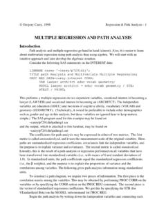
9 Figure 3 gives the path model for ARCHITCT. You should be able to calculate the direct and the indirect effects of the independent variables for this case. Figure 3. path model for variable ARCHTCT. Gregory Carey, 1998 Regression & path analysis - 5 Formal Tracing Rules Although we "intuited" the rules for path analysis above, there are formal tracing rules for calculating the correlations for a path diagram. First, pick a variable to start. It can be either the independent variable or the dependent variable. Then trace a route to the other variable, multiplying the coefficients when you go through two or more paths. Add together the results of these tracings for all the unique pathways. There are two exclusionary rules: (1) if you enter a variable on an arrowhead, you cannot exit on an arrowhead. Therefore, tracing from EDUC to VOCAB and then from VOCAB to GEOMETRY is illegal because we entered VOCAB on an arrowhead and exited VOCAB on an arrowhead.

10 But tracing from LAWYER to EDUC and then from EDUC to VOCAB is legal because we did not enter on EDUC on an arrowhead. (2) in any single pathway, you cannot go through the same variable twice. This rule is mentioned here for completeness. One will not encounter cases in a multiple regression path model where one could go through the same variable twice. Multivariate Multiple Regression & path analysis An astute person who examines the significance and values of the standardized beta weights and the correlations will quickly realize that interpretation through path analysis and interpretation of these weights give the same substantive conclusions. The chief advantage of path analysis is seen when there are two or more dependent variables. Technically, this is referred to as multivariate multiple regression. Here path analysis decomposes the sources of the correlations among the dependent variables.