Transcription of Probability and Random Processes - Chalmers
1 Probability and Random ProcessesSerik Sagitov, Chalmers University of Technology and Gothenburg UniversityAbstractLecture notes based on the book Probability and Random Processes by Geoffrey Grimmett andDavid Stirzaker. Last updated August 12, Random events and Probability space .. Conditional Probability and independence .. Random variables .. Random vectors .. Filtration ..62 Expectation and conditional Expectation .. Conditional expectation and prediction .. Multinomial distribution .. Multivariate normal distribution .. Sampling from a distribution .. Probability generating, moment generating, and characteristic functions .. Inequalities .. 123 Convergence of Random Borel-Cantelli lemmas .. Modes of convergence .. Continuity of expectation.
2 Weak law of large numbers .. Central limit theorem .. Strong LLN .. 174 Markov Simple Random walks .. Markov chains .. Stationary distributions .. Reversibility .. Poisson process and continuous-time Markov chains .. The generator of a continuous-time Markov chain .. 235 Stationary Weakly and strongly stationary Processes .. Linear prediction .. Linear combination of sinusoids .. The spectral representation .. Stochastic integral .. The ergodic theorem for the weakly stationary Processes .. The ergodic theorem for the strongly stationary Processes .. Gaussian Processes .. 316 Renewal theory and Renewal function and excess life .. LLN and CLT for the renewal process.
3 Stopping times and Wald s equation .. Stationary distribution .. Renewal-reward Processes .. Regeneration technique for queues .. M/M/1 queues .. M/G/1 queues .. G/M/1 queues .. G/G/1 queues .. 387 Definitions and examples .. Convergence inL2.. Doob s decomposition .. Hoeffding s inequality .. Convergence inL1.. Bounded stopping times. Optional sampling theorem .. Unbounded stopping times .. Maximal inequality .. Backward martingales. Strong LLN .. 498 Diffusion The Wiener process .. Properties of the Wiener process .. Examples of diffusion Processes .. The Ito formula .. The Black-Scholes formula .. 541 Random events and Probability spaceA Random experiment is modeled in terms of aprobability space( ,F,P) thesample space is the set of all possible outcomes of the experiment, the -field(or sigma-algebra)Fis a collection of measurable subsetsA (which are calledrandom events) satisfying1.
4 F,2. ifAi F, 0 = 1,2,.., then i=1Ai F, countable unions,3. ifA F, thenAc F,complementary event, the Probability measurePis a function onFsatisfying three Probability axioms1. ifA F, thenP(A) 0, ( ) = 1,3. ifAi F, 0 = 1,2,..are all disjoint, thenP( i=1Ai) = i=1P(Ai).2De Morgan s laws( iAi)c= iAci,( iAi)c= derived from the axiomsP( ) = 0,P(Ac) = 1 P(A),P(A B) =P(A) +P(B) P(A B).Inclusion-exclusion ruleP(A1 .. An) = iP(Ai) i<jP(Ai Aj) + i<j<kP(Ai Aj Ak) ..+ ( 1)n+1P(A1 .. An).Continuity of the Probability measure ifA1 A2 ..andA= i=1Ai= limi Ai, thenP(A) = limi P(Ai), ifB1 B2 ..andB= i=1Bi= limi Bi, thenP(B) = limi P(Bi). Conditional Probability and independenceIfP(B)>0, then the conditional Probability ofAgivenBisP(A|B) =P(A B)P(B).The law of total Probability and the Bayes formula. LetB1,..,Bnbe a partition of , thenP(A) =n i=1P(A|Bi)P(Bi),P(Bj|A) =P(A|Bj)P(Bj) ni=1P(A|Bi)P(Bi).
5 Definition ,..,Anare independent, if for any subset of events (Ai1,..,Aik)P(Ai1 .. Aik) =P(Ai1)..P(Aik).Example independence does not imply independence of three events. Toss two coins andconsider three events A={heads on the first coin}, B={tails on the first coin}, C={one head and one tail}.Clearly,P(A|C) =P(A) andP(B|C) =P(B) butP(A B|C) = Random variablesA real Random variable is a measurable functionX: Rso that different outcomes can givedifferent valuesX( ). Measurability ofX( ):{ :X( ) x} Ffor any real distributionPX(B) =P(X B) defines a new Probability space (R,B,PX), whereB= (allopen intervals) is the Borel function (cumulative distribution function)F(x) =FX(x) =PX{( ,x]}=P(X x).In terms of the distribution function we getP(a < X b) =F(b) F(a),P(X < x) =F(x ),P(X=x) =F(x) F(x ).Any monotone right-continuous function withlimx F(x) = 0 and limx F(x) = 1can be a distribution Random variableXis called discrete, if for some countable set of possible valuesP(X {x1,x2.))}
6 }) = distribution is described by the Probability mass functionf(x) =P(X=x).The Random variableXis called (absolutely) continuous, if its distribution has a Probability densityfunctionf(x):F(x) = x f(y)dy,for allx,so thatf(x) =F (x) almost indicator of a Random event 1A= 1{ A}withp=P(A) has a Bernoulli distributionP(1A= 1) =p,P(1A= 0) = 1 several eventsSn= ni=11 Aicounts the number of events that occurred. If independent eventsA1,A2,..have the same probabilityp=P(Ai), thenSnhas a binomial distribution Bin(n,p)P(Sn=k) =(nk)pk(1 p)n k, k= 0,1,.., (Cantor distribution) Consider ( ,F,P) with = [0,1],F=B[0,1], andP([0,1]) = 1P([0,1/3]) =P([2/3,1]) = 2 1P([0,1/9]) =P([2/9,1/3]) =P([2/3,7/9]) =P([8/9,1]) = 2 2and so on. PutX( ) = , its distribution, called the Cantor distribution, is neither discrete nor contin-uous. Its distribution function, called the Cantor function, is continuous but not absolutely Random vectorsDefinition joint distribution of a Random vectorX= (X1.
7 ,Xn) is the functionFX(x1,..,xn) =P({X1 x1} .. {Xn xn}).Marginal distributionsFX1(x) =FX(x, ,.., ),FX2(x) =FX( ,x, ,.., ),..FXn(x) =FX( ,.., ,x).4 The existence of the joint Probability density functionf(x1,..,xn) means that the distribution functionFX(x1,..,xn) = x1 .. xn f(y1,..,yn) ,for all (x1,..,xn),is absolutely continuous, so thatf(x1,..,xn) = nF(x1,..,xn) xnalmost variables (X1,..,Xn) are called independent if for any (x1,..,xn)P(X1 x1,..,Xn xn) =P(X1 x1)..P(Xn xn).In the jointly continuous case this equivalent tof(x1,..,xn) =fX1(x1)..fXn(xn).Example general, the joint distribution can not be recovered form the marginal distributions. IfFX,Y(x,y) =xy1{(x,y) [0,1]2},then vectors (X,Y) and (X,X) have the same marginal (x,y) = 1 e x xe yif 0 x y,1 e y ye yif 0 y x, thatF(x,y) is the joint distribution function of some pair (X,Y).
8 Find the marginal distributionfunctions and Three properties should be satisfied forF(x,y) to be the joint distribution function of somepair (X,Y) (x,y) is non-decreasing on both variables, (x,y) 0 asx andy , (x,y) 1 asx andy .Observe thatf(x,y) = 2F(x,y) x y=e y1{0 x y}is always non-negative. Thus the first property follows from the integral representation:F(x,y) = x y f(u,v)dudv,which, for 0 x y, is verifies as x y f(u,v)dudv= x0( yue vdv)du= 1 e x xe y,and for 0 y xas x y f(u,v)dudv= y0( yue vdv)du= 1 e y ye second and third properties are straightforward. We have shown also thatf(x,y) is the joint 0 andy 0 we obtain the marginal distributions as limitsFX(x) = limy F(x,y) = 1 e x, fX(x) =e x,FY(y) = limx F(x,y) = 1 e y ye y, fY(y) =ye Exp(1) andY Gamma(2,1).5H1T1T2H2H3H4T4H2T2H4H4H4H4H4 H4H4T4T4T4T4T4T4T4H3H3H3T3T3T3T3F1F2F3F4 F5 Figure 1: Filtration for four consecutive coin FiltrationDefinition sequence of sigma-fields{Fn} n=1such thatF1 F2.
9 Fn ..,Fn Ffor allnis called a illustrate this definition use an infinite sequence of Bernoulli trials. LetSnbe the number of headsinnindependent tossings of a fair coin. Figure 1 shows imbedded partitionsF1 F2 F3 F4 F5of the sample space generated byS1,S2,S3,S4, events representing our knowledge of the first three tossings is given byF3. From the perspectiveofF3we can not say exactly the value ofS4. Clearly, there is dependence betweenS3andS4. The jointdistribution ofS3andS4:S4= 0S4= 1S4= 2S4= 3S4= 4 TotalS3= 01/161/160001/8S3= 103/163/16003/8S3= 2003/163/1603/8S3= 30001/161/161/8 Total1/161/43/81/41/161 The conditional expectationE(S4|S3) =S3+ a discrete Random variable with values , , , and probabilities 1/8,3/8,3/8,1 finitenthe picture is straightforward. Forn= it is a non-trivial task to define an overall( ,F,P) with = (0,1].)
10 One can use the Lebesgue measureP(dx) =dxand the sigma-fieldFofLebesgue measurable subsets of (0,1]. Not all subsets of (0,1] are Lebesgue Expectation and conditional ExpectationThe expected value ofXisE(X) = X( )P(d ).A discrete a finite number of possible values is a simple in thatX=n i=1xi1Ai6for some partitionA1,..,Anof . In this case the meaning of the expectation is obviousE(X) =n i=1xiP(Ai).For any non-negative are simple such thatXn( ) X( ) for all , and theexpectation is defined as a possibly infinite limitE(X) = limn E(Xn).Any be written as a difference of two non-negative +=X 0 andX = X at least one ofE(X+) andE(X ) is finite, thenE(X) =E(X+) E(X ), otherwiseE(X) does discrete with the Probability mass functionf(k) =12k(k 1)fork= 1, 2, 3,..has no a discrete mass functionfand any functiongE(g(X)) = xg(x)f(x).))