Transcription of Random Variables, Distributions, and Expected Value
1 Random Variables, Distributions, and Expected ValueFall 2001 Professor Paul GlassermanB6014: Managerial Statistics403 Uris HallThe Idea of a Random Variable1. Arandom variableis a variable that takes specific values with specific can be thought of as a variable whose Value depends on the outcome of an We usually denote Random variables by capital letters near the end of the alphabet; ,X,Y, Example: LetXbe the outcome of the roll of a die. ThenXis a Random variable . Itspossible values are 1, 2, 3, 4, 5, and 6; each of these possible values has probability 1 The word Random in the term Random variable doesnotnecessarily imply that theoutcome is completely Random in the sense that all values are equally likely. Some valuesmay be more likely than others; Random simply means that the Value is When you think of a Random variable , immediately ask yourself What are the possible values? What are their probabilities?6. Example: LetYbe thesumof two dice rolls.
2 Possible values:{2,3,4,..,12}. Their probabilities: 2 has probability 1/36, 3 has probability 2/36, 4 has probability3/36, etc. (The important point here is not the probabilities themselves, but ratherthe fact that such a probability can be assigned to each possible Value .)7. The probabilities assigned to the possible values of a Random variable are distribution completely describes a Random A Random variable is calleddiscreteif it has countably many possible values; otherwise,it is example, if the possible values are any of these: {1,2,3,..,} {.., 2, 1,0,1,2,..} {0,2,4,6,..} {0, , , , ,..} any finite setthen the Random variable is discrete. If the possible values are any of these: all numbers between 0 and all numbers between and all numbers between 0 and 1then the Random variable is continuous. Sometimes, we approximate a discrete randomvariable with a continuous one if the possible values are very close together; , stockprices are often treated as continuous Random The following quantities would typically be modeled as discrete Random variables: The number of defects in a batch of 20 items.
3 The number of people preferring one brand over another in a market research study. The credit rating of a debt issue at some date in the following would typically be modeled as continuous Random variables: The yield on a 10-year Treasury bond three years from today. The proportion of defects in a batch of 10,000 items. The time between breakdowns of a Distributions1. The rule that assigns specific probabilities to specific values for a discrete Random variableis called itsprobability mass a discrete Random variable thenwe denote its pmf byPX. For any valuex,P(X=x) is the probability of the event thatX=x; ,P(X=x) = probability that the Value Example: IfXis the outcome of the roll of a die, thenP(X=1)=P(X=2)= =P(X=6)=1/6,andP(X=x) = 0 for all other values 3 2 1 1: Left panel shows the probability mass function for the sum of two dice; the possiblevalues are 2 through 12 and the heights of the bars give their probabilities.
4 The bar heightssum to 1. Right panel shows a probability density for a continuous Random variable . TheprobabilityP(1<X ) is given by the shaded area under the curve betwee 1 and Thetotal area under the curve is 1. The probability of any particular Value , ,P(X= 1) is zerobecause there is no area under a single NOTE: We always use capital letters for Random variables. Lower-case letters likexandystand for possible values ( , numbers) and are not A pmf is graphed by drawing a vertical line of heightP(X=x) at each possible is similar to a histogram, except that the height of the line (or bar) gives thetheoreticalprobabilityrather than theobserved Distributions1. The distribution of a continuous Random variable cannot be specified through a probabilitymass function because ifXis continuous, thenP(X=x) = 0 for allx; , the probabilityof any particular Value is zero. Instead, we must look at probabilities ofrangesof The probabilities of ranges of values of a continuous Random variable are determined by adensityfunction.
5 The density ofXis denoted byfX. The area under a density is always1. The probability thatXfalls between two pointsaandbis the area underfXbetweenthe pointsaandb. The familiar bell-shaped curve is an example of a Thecumulative distribution functionorcdfgives the probability that a randomvariableXtakes values less than or equal to a given valuex. Specifically, the cdf ofX,denoted byFX,isgivenbyFX(x)=P(X x).So,FX(x) is the area under the densityfXto the left For a continuous Random variable ,P(X=x) = 0; consequently,P(X x)=P(X<x).For a discrete Random variable , the two probabilities are not in general The probability thatXfalls between two pointsaandbis given by the difference betweenthe cdf values at these points:P(a<X b)=FX(b) FX(a).SinceFX(b) is the area underfXto the left ofband sinceFX(a) is the area underfXtothe left ofa, their difference is the area underfXbetween the two of Random Variables1. Theexpected valueof a Random variable is denoted byE[X].
6 The Expected valuecan be thought of as the average Value attained by the Random variable ; in fact, theexpected Value of a Random variable is also called itsmean, in which case we use thenotation X.( is the Greek letter mu.)2. The formula for the Expected Value of a discrete Random variable is this:E[X]= all possiblexxP(X=x).In words, the Expected Value is the sum, over all possible valuesx,ofxtimes its probabilityP(X=x).3. Example: The Expected Value of the roll of a die is1(16)+2(16)+3(16)+ +6(16)=21/6= that the Expected Value is not one of the possible outcomes: you can t roll a , if you average the outcomes of a large number of rolls, the result We also define the Expected Value for a function of a Random variable . Ifgis a function(for example,g(x)=x2), then the Expected Value ofg(X)isE[g(X)] = all possiblexg(x)P(X=x).For example,E[X2]= all possiblexx2P(X=x).In general,E[g(X)] is not the same asg(E[X]). In particular,E[X2] is not the same as(E[X]) The Expected Value of a continuous Random variable cannot be expressed as a sum; insteadit is an integral involving the density.
7 (If you don t know what that means, don t worry;we won t be calculating any integrals.)46. Thevarianceof a Random variableXis denoted by eitherVar[X]or 2X.( is the Greekletter sigma.) The variance is defined by 2X=E[(X X)2];this is the Expected Value of the squared difference betweenXand its mean. For a discretedistribution, we can write the variance as 2X= x(x X)2P(X=x).7. An alternative expression for the variance (valid for both discrete and continuous randomvariables) is 2X=E[(X2)] ( X) is the difference between the Expected Value ofX2and the square of the mean Thestandard deviationof a Random variable is the square-root of its variance andis denoted by X. Generally speaking, the greater the standard deviation, the morespread-out the possible values of the Random In fact, there is a Chebyshe vrule for Random variables: ifm>1, then the probabilitythatXfalls withinmstandard deviations of its mean is at least 1 (1/m2); that is,P( x m X X X+m X) 1 (1/m2).
8 10. Find the variance and standard deviation for the roll of one die. Solution: We use theformulaVar[X]=E[X2] (E[X])2. We found previously thatE[X]= , so now weneed to findE[X2]. This is given byE[X2]=6 x=1x2PX(x)=12(16)+22(16)+ +62(16)= , 2X=Var[X]=E[X2] (E[X])2= ( )2= = = Transformations of Random Variables1. IfXis a Random variable and ifaandbare any constants, thena+bXis shifts it bya. A linear transformation ofXis another Random variable ; we often denote it Example: Suppose you have investments in Japan. The Value of your investment (in yen)one month from today is a Random variableX. Suppose you can convert yen to dollarsat the rate ofbdollars per yen after paying a commission ofadollars. What is the valueof your invenstment, in dollars, one month from today? Answer: a+ Example: Your salary isadollars per year. You earn a bonus ofbdollars for every dollarof sales you bring in. IfXis what you sell, how much do you make?
9 4. Example: It takes you exactly 16 minutes to walk to the train station. The train ridetakesXhours, whereXis a Random variable . How long is your trip, in minutes?5. IfZ=a+bX,thenE[Z]=E[a+bX]=a+bE[X]=a+b Xand 2Z=Var[a+bX]=b2 Thus, the Expected Value of a linear transformation ofXis just the linear transformationof the Expected Value ofX. Previously, we said thatE[g(X)] andg(E[X]) are generallydifferent. Theonlycase in which they are the same is whengis a linear transformation:g(x)=a+ Notice that the variance ofa+bXdoes not depend ona. This is appropriate: thevariance is a measure of spread; addingadoes not change the spread, it merely shifts thedistribution to the left or to the Distributed Random Variables1. So far, we have only considered individual Random variables. Now we turn to propertiesof several Random variables considered at the same time. The outcomes of these differentrandom variables may be Examples(a) Think of the price of each stock in the New York exchange as a Random variable ; themovements of these variables are related.
10 (b) You may be interested in the probability that a randomly selected shopper buysprepared frozen meals. In designing a promotional campaign you might be evenmore interested in the probability that that same shopper also buys instant coffeeand reads a certain magazine.(c) The number of defects produced by a machine in an hour is a Random variable . Thenumber of hours the machine operator has gone without a break is another randomvariable. You might well be interested in probabilities involving these two randomvariables The probabilities associated with multiple Random variables are determined by with individual Random variables, we distinguish discrete and contin-uous In the discrete case, the distribution is determined by ajoint probability mass func-tion. For example, ifXandYare Random variables, there joint pmf isPX,Y(x,y)=P(X=x,Y=y)= probability thatX=xandY= several Random variablesX1,..,Xn,wedenotethejointpmfbyP X1,.., It is often convenient to represent a joint pmf through a table.