Transcription of Reading 5b: Continuous Random Variables
1 Continuous Random Variables Class 5, Jeremy Orloff and Jonathan Bloom 1 Learning Goals 1. Know the definition of a Continuous Random variable. 2. Know the definition of the probability density function (pdf) and cumulative distribution function (cdf). 3. Be able to explain why we use probability density for Continuous Random Variables . 2 Introduction We now turn to Continuous Random Variables . All Random Variables assign a number to each outcome in a sample space. Whereas discrete Random Variables take on a discrete set of possible values, Continuous Random Variables have a Continuous set of values.
2 Computationally, to go from discrete to Continuous we simply replace sums by integrals. It will help you to keep in mind that (informally) an integral is just a Continuous sum. Example 1. Since time is Continuous , the amount of time Jon is early (or late) for class is a Continuous Random variable. Let s go over this example in some detail. Suppose you measure how early Jon arrives to class each day (in units of minutes). That is, the outcome of one trial in our experiment is a time in minutes. We ll assume there are Random fluctuations in the exact time he shows up.
3 Since in principle Jon could arrive, say, minutes early, or minutes late (corresponding to the outcome ), or at any other time, the sample space consists of all real numbers. So the Random variable which gives the outcome itself has a Continuous range of possible values. It is too cumbersome to keep writing the Random variable , so in future examples we might write: Let T = time in minutes that Jon is early for class on any given day. 3 Calculus Warmup While we will assume you can compute the most familiar forms of derivatives and integrals by hand, we do not expect you to be calculus whizzes.
4 For tricky expressions, we ll let the computer do most of the calculating. Conceptually, you should be comfortable with two views of a definite integral. b (x) dx = area under the curve y = f(x). a b (x) dx = sum of f(x) dx . a 1 2 4 class 5, Continuous Random Variables , Spring 2014 The connection between the two is: nn area sum of rectangle areas = f(x1) x + f(x2) x + .. + f(xn) x = f(xi) x. 1 As the width x of the intervals gets smaller the approximation becomes better. xyaby=f(x)xyx0x1x2xn x aby=f(x)Area =f(xi) xArea is approximately the sum of rectangles Note: In calculus you learned to compute integrals by finding antiderivatives.
5 This is important for calculations, but don t confuse this method for the reason we use integrals. Our interest in integrals comes primarily from its interpretation as a sum and to a much lesser extent its interpretation as area. Continuous Random Variables and Probability Density Func tions A Continuous Random variable takes a range of values, which may be finite or infinite in extent. Here are a few examples of ranges: [0, 1], [0, ), ( , ), [a, b]. Definition: A Random variable X is Continuous if there is a function f(x) such that for any c d we have d P (c X d) = f(x) dx.]
6 (1) c The function f(x) is called the probability density function (pdf). The pdf always satisfies the following properties: 1. f(x) 0 (f is nonnegative). 2. f(x) dx = 1 (This is equivalent to: P ( < X < ) = 1). The probability density function f(x) of a Continuous Random variable is the analogue of the probability mass function p(x) of a discrete Random variable. Here are two important differences: 1. Unlike p(x), the pdf f(x) is not a probability. You have to integrate it to get proba bility. (See section below.) 2. Since f(x) is not a probability, there is no restriction that f(x) be less than or equal to 1.
7 Class 5, Continuous Random Variables , Spring 2014 3 Note: In Property 2, we integrated over ( , ) since we did not know the range of values taken by X. Formally, this makes sense because we just define f(x) to be 0 outside of the range of X. In practice, we would integrate between bounds given by the range of X. Graphical View of Probability If you graph the probability density function of a Continuous Random variable X then P (c X d) = area under the graph between c and d. xf(x)cdP(c X d)Think: What is the total area under the pdf f(x)?
8 The terms probability mass and probability density Why do we use the terms mass and density to describe the pmf and pdf? What is the difference between the two? The simple answer is that these terms are completely analogous to the mass and density you saw in physics and calculus. We ll review this first for the probability mass function and then discuss the probability density function. Mass as a sum: If masses m1, m2, m3, and m4 are set in a row at positions x1, x2, x3, and x4, then the total mass is m1 + m2 + m3 + m4. m1 m2 m3 m4 x x1 x2 x3 x4 We can define a mass function p(x) with p(xj ) = mj for j = 1, 2, 3, 4, and p(x) = 0 otherwise.
9 In this notation the total mass is p(x1) + p(x2) + p(x3) + p(x4). The probability mass function behaves in exactly the same way, except it has the dimension of probability instead of mass. Mass as an integral of density: Suppose you have a rod of length L meters with varying density f(x) kg/m. (Note the units are mass/length.) x x x1 x2 x3 xi0 xn = L mass of ith piece f(xi) x class 5, Continuous Random Variables , Spring 2014 4 If the density varies continuously, we must find the total mass of the rod by integration: L total mass = f(x) dx. 0 This formula comes from dividing the rod into small pieces and summing up the mass of each piece.
10 That is: nn total mass f(xi) x i=1 In the limit as x goes to zero the sum becomes the integral. The probability density function behaves exactly the same way, except it has units of probability/(unit x) instead of kg/m. Indeed, equation (1) is exactly analogous to the above integral for total mass. While we re on a physics kick, note that for both discrete and Continuous Random Variables , the expected value is simply the center of mass or balance point. Example 2. Suppose X has pdf f(x) = 3 on [0, 1/3] (this means f(x) = 0 outside of [0, 1/3]). Graph the pdf and compute P (.)