Refrigeration Basics and LNG - University of Oklahoma

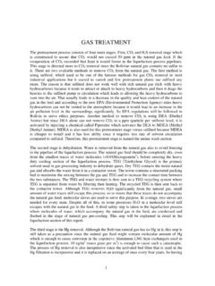
1 56 Refrigeration CYCLES Carnot Cycle We start discussing the well-known Carnot cycle in its Refrigeration mode. Figure 2-1: Carnot Cycle In this cycle we define the coefficient of performance as follows: LLHLqTCOPwT T== (2-1) Which comes from the fact that HLwq q= (first law) and LLqTs= , HHqTs= (second law). Note that w is also given by the area of the rectangle. Temperature differences make the COP vary. For example, the next figure shows how COP varies with TL (TH is ambient in this case) and the temperature difference in exchangers.

2 57 Figure 2-2: COP changes with heat exchanger temperature approximation and TL (TH=ambient) We now turn our attention to a real one stage Refrigeration cycle, depicted in the next figure. Figure 2-3: Typical one-stage dry Refrigeration Cycle We notice that: - To be able to achieve the best match possible with the rectangular shape it is necessary to operate inside the two phase region. - Compression is in this example performed outside the two phase region. Creating a horn , which is not thermodynamically advisable, is mechanically better.

3 For this reason, this cycle is called dry cycle. A wet cycle is shown in the next figure. 58 Figure 2-4: Wet Refrigeration Cycle - The expander has been substituted by a throttling valve. If an expander had been used the line from d to a would be a vertical line. This is also done for mechanical reasons. The Refrigeration cycles can also be represented in a P-H diagram. Figure 2-5: P-H diagram representation of a dry Refrigeration cycle 59 Exercise 2-1: Consider the real cycle taking place outside the two phase region using a compressor and an expander.

4 This is called, the Bryton Cycle. Prove that this cycle is less efficient than the Carnot cycle. To do this assume constant Cp Exercise 2-2: Consider the real dry Refrigeration cycle. Prove that the area of inside the cycle plus the shaded area (called throttling loss) is equal to the total work. Show also that this is less efficient than the pure Carnot cycle. Refrigerant fluid choice: We now turn our attention to the fluids. Usually, one tends to pick pL as low as possible, but not below atmospheric pressure.

5 Thus, the refrigerant chosen needs to have a normal boiling point compatible with the lowest temperature of the cycle (usually 10oC lower than the system one wants to cool). The higher pressure needs to be compatible with the cooling media used for qH. If this is cooling water , then the TH needs to be around 10oC higher than the available cooling water temperature. The next table shows the existing refrigerants. It is followed by the boiling temperature and rang of selected refrigerants. 60 Table 2-1: Refrigerants 61 Table 2-1: Refrigerants Continued) 62 Table 2-1: Refrigerants Continued) 63 Figure 2-6: Temperature Ranges of Refrigerants We now turn to Pro II to show how a refrigerant cycle is built.

6 We start with entering the cycle as follows: 64We pick R12, which will allow us to cool down anything to Next we define the outlet pressure of the compressor. This needs to be such that stream C (after the cooler) is higher than 60 oF. To start we choose around 85 psia. Next we define the top heat exchanger, by specifying an outlet temperature slightly below the bubble point. 65 We continue by specifying the duty of the bottom exchanger. This is customary because this is the targeted design goal of the cycle.

7 66 We enter the outlet pressure of the valve (atmospheric). 67 We also realize that this flowsheet does not have input or output streams. Thus, to start the simulation, one needs to give an initial value to a stream. We chose stream D, and initialize with a flowrate that is guessed. 68 If the flowrate chosen is too high, then the inlet of the compressor will be two phase and this is not advisable. If the flowrate is too low, the cycle will loose efficiency (the horn will get larger).

8 Warning: Pro II may not realize internally that it needs to solve the unit that the initialized stream feeds to and try to continue until it reaches convergence in the loop but it will loose the input data. To avoid problems we specify the order in which we want the flowsheet to solve by clicking in the unit sequence button. 69 Exercise 2-3: Construct the simulation above described and determine the right flowrate in the cycle. Determine all temperatures and obtain the COP. Compare it with a Carnot Cycle.

9 The above exercise can be done automatically using a controller , which is a type of spec and vary equivalent to Goal Seek in Excel. Once the controller is picked, double clicking on it reveals the menu. 70 Thus, we choose to have the inlet to the compressor just slightly above dew point (specification) and we vary the flowrate, just as we did by hand. It is, however, easier to specify a very low liquid fraction. Make sure the starting point is close to the right value.

10 Sometimes the controller has a hard time converging. 71 We now turn our attention to a variant where liquid is being sub-cooled: Figure 2-7: Liquid sub-cooling in a Refrigeration cycle. 72 The corresponding TS and P-H diagrams are shown in the next figure. Since we are using the vapor (at the lower pressure) to sub-cool, there is a gain in qL at the expense of a slight increase in work. Whether there is a gain, it depends on the fluid and the sub-cooled temperature choice. Figure 2-8: TS and P-H diagram for liquid sub-cooling in a Refrigeration cycle.