Transcription of Regression Analysis: A Complete Example
1 Regression Analysis: A Complete Example This section works out an Example that includes all the topics we have discussed so far in this chapter. A Complete Example of Regression analysis. PhotoDisc, Images A random sample of eight drivers insured with a company and having similar auto insurance policies was selected. The following table lists their driving experiences (in years) and monthly auto insurance premiums. Driving Experience (years) Monthly Auto Insurance Premium 5 $64 2 87 12 50 9 71 15 44 6 56 25 42 16 60 a. Does the insurance premium depend on the driving experience or does the driving experience depend on the insurance premium?
2 Do you expect a positive or a negative relationship between these two variables? b. Compute SSxx, SSyy, and SSxy. c. Find the least squares Regression line by choosing appropriate dependent and independent variables based on your answer in part a. d. Interpret the meaning of the values of a and b calculated in part c. e. Plot the scatter diagram and the Regression line. f. Calculate r and r2 and explain what they mean. g. Predict the monthly auto insurance premium for a driver with 10 years of driving experience. h. Compute the standard deviation of errors. i. Construct a 90% confidence interval for B. j. Test at the 5% significance level whether B is negative.
3 K. Using = .05, test whether is different from zero. Solution a. Based on theory and intuition, we expect the insurance premium to depend on driving experience. Consequently, the insurance premium is a dependent variable and driving experience is an independent variable in the Regression model. A new driver is considered a high risk by the insurance companies, and he or she has to pay a higher premium for auto insurance. On average, the insurance premium is expected to decrease with an increase in the years of driving experience. Therefore, we expect a negative relationship between these two variables. In other words, both the population correlation coefficient and the population Regression slope B are expected to be negative.
4 B. Table shows the calculation of x, y, xy, x2, and y2. Table Experience x Premium y xy x2 y2 5 64 320 25 4096 2 87 174 4 7569 12 50 600 144 2500 9 71 639 81 5041 15 44 660 225 1936 6 56 336 36 3136 25 42 1050 625 1764 16 60 960 256 3600 x = 90 y = 474 xy = 4739 x2 = 1396 y2 = 29,642 The values of x and y are The values of SSxy, SSxx, and SSyy are computed as follows: c. To find the Regression line, we calculate a and b as follows: Thus, our estimated Regression line = a + bx is d. The value of a = gives the value of for x = 0; that is, it gives the monthly auto insurance premium for a driver with no driving experience.
5 However, as mentioned earlier in this chapter, we should not attach much importance to this statement because the sample contains drivers with only two or more years of experience. The value of b gives the change in due to a change of one unit in x. Thus, b = indicates that, on average, for every extra year of driving experience, the monthly auto insurance premium decreases by $ Note that when b is negative, y decreases as x increases. e. Figure shows the scatter diagram and the Regression line for the data on eight auto drivers. Note that the Regression line slopes downward from left to right. This result is consistent with the negative relationship we anticipated between driving experience and insurance premium.
6 Figure Scatter diagram and the Regression line. f. The values of r and r2 are computed as follows: The value of r = .77 indicates that the driving experience and the monthly auto insurance premium are negatively related. The (linear) relationship is strong but not very strong. The value of r2 = .59 states that 59% of the total variation in insurance premiums is explained by years of driving experience and 41% is not. The low value of r2 indicates that there may be many other important variables that contribute to the determination of auto insurance premiums. For Example , the premium is expected to depend on the driving record of a driver and the type and age of the car.
7 G. Using the estimated Regression line, we find the predicted value of y for x = 10 is Thus, we expect the monthly auto insurance premium of a driver with 10 years of driving experience to be $ h. The standard deviation of errors is i. To construct a 90% confidence interval for B, first we calculate the standard deviation of b: For a 90% confidence level, the area in each tail of the t distribution is The degrees of freedom are From the t distribution table, the t value for .05 area in the right tail of the t distribution and 6 df is The 90% confidence interval for B is Thus, we can state with 90% confidence that B lies in the interval to.
8 52. That is, on average, the monthly auto insurance premium of a driver decreases by an amount between $.52 and $ for every extra year of driving experience. j. We perform the following five steps to test the hypothesis about B. Step 1. State the null and alternative hypotheses. The null and alternative hypotheses are written as follows: Note that the null hypothesis can also be written as H0: B 0. Step 2. Select the distribution to use. Because is not known, we use the t distribution to make the hypothesis test. Step 3. Determine the rejection and nonrejection regions. The significance level is .05. The < sign in the alternative hypothesis indicates that it is a left-tailed test.
9 From the t distribution table, the critical value of t for .05 area in the left tail of the t distribution and 6 df is , as shown in Figure Figure Step 4. Calculate the value of the test statistic. The value of the test statistic t for b is calculated as follows: Step 5. Make a decision. The value of the test statistic t = falls in the rejection region. Hence, we reject the null hypothesis and conclude that B is negative. That is, the monthly auto insurance premium decreases with an increase in years of driving experience. Using the p-Value to Make a Decision We can find the range for the p-value from the t distribution table (Table V of Appendix C) and make a decision by comparing that p-value with the significance level.
10 For this Example , df = 6 and the observed value of t is From Table V (the t distribution table) in the row of df = 6, is between and The corresponding areas in the right tail of the t distribution are .025 and .01. But our test is left-tailed and the observed value of t is negative. Thus, t = lies between and The corresponding areas in the left tail of the t distribution are .025 and .01. Therefore the range of the p-value is .01 < p-value<.025 Thus, we can state that for any equal to or greater than .025 (the upper limit of the p-value range), we will reject the null hypothesis. For our Example , = .05, which is greater than the upper limit of the p-value of.