Repeated Measures ANOVA - Stony Brook

1 Repeated Measures ANOVA Prof. Wei Zhu Department of Applied Mathematics & Statistics Stony Brook University 2 The One-way ANOVA we have just learnt can test the equality of several population means. It is an extension of the pooled variance t-test That is: H0 (null hypothesis) : 1 = 2 = 3 =.. = k Ha (alternative hypothesis): At least one of means differs from the rest. Assumptions: Unknown but equal population variances Normal populations Independent samples 3 The F statistic kinjiijkNkiiikjxxxxnF11211211where xij = the jth observation in the i th sample. injki,,2,1 and ,,2,1 kiinxxthinjijii,,2,1 sample for mean 1 size sample Total 1 kiinNmean Overall 11 Nxxkinjiji4 The ANOVA table kiiiBxxnSS12 WBMSMSF kiiikBxxnMS1211 kinjiijWjxxSS112 kinjiijkNWjxxMS11211 kkN Source , F Between Within The ANOVA table is a tool for displaying the computations for the F test.

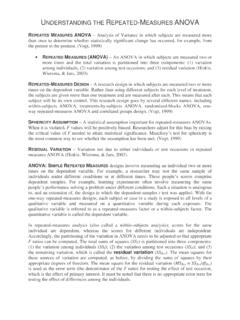
2 It is very important when the Between Sample variability is due to two or more factors. We reject the ANOVA null hypothesis of equal means if F > Fk-1,N-k, 5 The most distinct disadvantage to the analysis of variance ( ANOVA ) method is that it requires three assumptions to be made: The samples must be independent to each other. All variances from each data group, though unknown, must be normality assumption. Limitations of the one-way ANOVA : 6 7 A Repeated Measures design is one in which at least one of the factors consists of Repeated measurements on the same subjects or experimental units, under different conditions and/or at different time points. 8 A Repeated Measures design often involves measuring subjects at different points in time or subjects measured under different experimental conditions It can be viewed as an extension of the paired-samples t-test (which involved only two related Measures ) Thus, the Measures unlike in the regular ANOVA are correlated, that is, the observations are not independent 9 Example: Data collected in a sequence of (often) evenly spaced points in time this is usually referred to as the longitudinal data Example: Different treatments are assigned to the each experimental unit 10 By collecting data from the same participants under Repeated conditions, the individual differences can be eliminated or reduced as a source of between group differences.

3 Also, the sample size is not divided between conditions or groups and thus inferential testing becomes more powerful. This design also proves to be economical when sample members are difficult to recruit. 11 12 As with any ANOVA , Repeated Measures ANOVA tests the equality of means. However, Repeated Measures ANOVA is used when all members of a random sample are measured under a number of different conditions or at different time points. As the sample is exposed to each condition, the measurement of the dependent variable is Repeated . Using a standard ANOVA in this case is not appropriate because it fails to model the correlation between the Repeated Measures : the data violate the ANOVA assumption of independence. 13 The simplest example of a Repeated Measures design is a paired samples t-test: Each subject is measured twice, for example, time 1 and time 2, on the same variable; or, each pair of matched participants are assigned to two treatment levels.

4 If we observe participants at more than two time-points, then we need to conduct a Repeated Measures ANOVA . 14 What we would like to do is to decompose the variability into (1) A random subject effect (2) A fixed treatment or time effect Treating the subject as a random effect has the added advantage that we can extend our conclusion to the population where these subjects were drawn from. 15 Yij = j +Si+ ij j = The fixed effect, j=1, ,k Si= The random effect of subject i, i=1, ,n ij = The random error independent of Si Furthermore, we set the total number of observations as: N = n*k 16 17 17 18 We will reject the ANOVA null hypothesis if Fk-1,(k-)(n-1) > 19 20 Assumptions summary: For a Repeated Measures design, we start with the same assumptions as a paired samples t-test : Participants are independent and randomly selected from the population Normality Then, very importantly, there are two approaches to Repeated Measures ANOVA depends on the assumption of the variance-covariance matrix: the univariate approach (where compound symmetry is imposed), and the multivariate approach (where no assumption is imposed) 21 Example: Consider the following experiment.

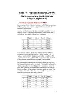
5 We have four drugs (1,2,3 and 4) that relieve pain. Each subject is given each of the four drugs. The subject s pain tolerance is then measured. Enough time is allowed to pass between successive drug administrations so that we can be sure there is no residual effect from the previous drug. The null hypothesis is: Mean(1)=Mean(2)=Mean(3)=Mean(4) 22 Subject Drug1 Drug2 Drug 3 Drug 4 1 5 9 6 11 2 7 12 8 9 3 11 12 10 14 4 3 8 5 8 Table: Pain tolerance under 4 different drugs 23 In the one-way analysis of variance without a Repeated measure , we would have each subject receive only one of the four drugs. In this design, each subjects is measured under each of the drug conditions. This has several important advantages as enumerated before. 24 Each subject acts as his own control. : drugs effects are calculated by recording deviations between each drug score and the average drug score for each subject.

6 The normal subject-to-subject variation can thus be removed from the error sum of squares. 25 26 27 SAS code using the Repeated Statement DATA REPEAT; INPUT SUBJ PAIN1-PAIN4; DATALINES; 1 5 9 6 11 2 7 12 8 9 3 11 12 10 14 4 3 8 5 8 ; PROC ANOVA DATA=REPEAT; TITLE 'using Repeated statement'; MODEL PAIN1-PAIN4 = / NOUNI; Repeated DRUG 4 (1 2 3 4) / printe; RUN; 28 Please see Quiz 3 solutions for detailed explanations of the SAS output. SAS code using the Repeated Statement Remark 1 : about the data set We need the data set in the form: SUBJ PAIN1 PAIN2 PAIN3 PAIN4 NOTICE that it does not have a DRUG variable 29 SAS code using the Repeated Statement Remark 2 : about the Repeated Statement The general form: Repeated factor_name CONTRAST(n); To compute pairwise comparisons N is a number from 1 to k, with k being # levels of Repeated factor; To get all pairwise contrasts, we need k-1 Repeated statements 30 SAS code using the Repeated Statement Remark 2 : about the Repeated Statement In our example: PROC ANOVA DATA=REPEAT; TITLE 'using Repeated statement'; MODEL PAIN1-PAIN4 = / NOUNI; Repeated DRUG 4 CONTRAST(1) / SUMMARY; Repeated DRUG 4 CONTRAST(2) / SUMMARY; Repeated DRUG 4 CONTRAST(3) / SUMMARY; RUN.

7 Request ANOVA tables for each contrast 31 SAS code using the Repeated Statement Remark 3 : more explanation of the ANOVA procedure PROC ANOVA DATA=REPEAT; TITLE 'using Repeated statement'; MODEL PAIN1-PAIN4 = / NOUNI; Repeated DRUG 4 (1 2 3 4) / printe; RUN; No CLASS: our data set does not have an independent variable NOUNI: not to conduct a separate analysis for each of the four PAIN 4: the Repeated factor DRUG has four levels; optional (1 2 3 4): the labels we want printed for each level of DRUG printe calls for the Machly s Sphericity Test for compound symmetry 32 SAS code using the Repeated Statement Remark 4 : Data conversion: the long form & the broad form DATA PAIN; INPUT SUBJ DRUG PAIN; DATALINES; 1 1 5 1 2 9 1 3 6 1 4 11 2 1 7 2 2 12 .. ; DATA PAIN; INPUT SUBJ @; DO DRUG = 1 to 4; INPUT PAIN @; OUTPUT; END; DATALINES; 1 5 9 6 11 2 7 12 8 9 3 11 12 10 14 4 3 8 5 8 ; DATA REPEAT; INPUT SUBJ PAIN1-PAIN4; DATALINES; 1 5 9 6 11 2 7 12 8 9 3 11 12 10 14 4 3 8 5 8 ; The following is the data format, the broad form, that You should master first.

8 33 Generate data in long form from the broad form DATA PAIN; INPUT SUBJ @; DATALINES; DO DRUG = 1 to 4; INPUT PAIN @; OUTPUT; END; iterative loop To keep reading from the same line of data 1 5 9 6 11 2 7 12 8 9 3 11 12 10 14 4 3 8 5 8 ; The broad form! The long form! 34 SAS: The DO loop the general form: Do variable = start TO end BY increment; (SAS Statements) END; initial value ending value Default: 1 35 in our example: initial value: 1 ending value: 4 DO DRUG = 1 to 4; INPUT PAIN @; OUTPUT; END; to keep reading from the same line of datareturn to DO SAS: The DO loop 36 Repeated measure / Longitudinal data: broad form 37 id time1 time2 time3 time4 1 31 29 15 26 2 24 28 20 32 3 14 20 28 30 4 38 34 30 34 5 25 29 25 29 6 30 28 16 34 Hypothetical data from Twisk, chapter 3, page 26, table Jos W.

9 R. Twisk. Applied Longitudinal Data Analysis for Epidemiology: A Practical Guide. Cambridge University Press, 2003. Repeated measure / Longitudinal data: Long form 38 Hypothetical data from Twisk, chapter 3, page 26, table id time score 1 1 31 1 2 29 1 3 15 1 4 26 2 1 24 2 2 28 2 3 20 2 4 32 3 1 14 3 2 20 3 3 28 3 4 30 id time score 4 1 38 4 2 34 4 3 30 4 4 34 5 1 25 5 2 29 5 3 25 5 4 29 6 1 30 6 2 28 6 3 16 6 4 34 Another way to convert data from broad form to long form in SAS: 39 data long; set broad; time=1; score=time1; output; time=2; score=time2; output; time=3; score=time3; output; time=4; score=time4; output; run.

10 The long form is used to plot the profile plot in the same way as the usual ANOVA 40 1 80 83 2 85 86 3 83 88 4 82 94 5 87 93 6 84 98 Subject Control Treatment PRE POST Factor B: TIME Factor A: GROUP Repeated 41 42 43 Total Variance df=N-1 Between subjects Within subjects Treatment df=a-1 Error due to subjects within treatment df=a(n-1) Time df=b-1 Treatment time df =(a-1) (b-1) Error or residual df =a (n-1) (b-1) a: # of treatment groups b: # of time points n: # of subjects per treatment N=a b n: total # of measurements 44 Source SS MS Factor A a-1 SSA MSA = SSA/(a-1) Factor B b-1 SSB MSB = SSB/(b-1) AB interaction (a-1)(b-1) SSAB MSAB = SSAB/(a-1)(b-1) Subjects (within A) a(n-1) SSWA MSWA = SSWA/a(n-1) Error a(n-1)(b-1) SSE MSE = SSE/a(n-1)(b-1) Total nab-1 SST 45 46 Data prepost; Input subj group $ pretest postest; datalines; 1 c 80 83 2 c 85 86 3 c 83 88 4 t 82 94 5 t 87 93 6 t 84 98 ; run; proc ANOVA data=prepost; title 'Two-way ANOVA with a Repeated measure on One Factor'; class group; model pretest postest = group/nouni; Repeated time 2 (0 1); run.