Transcription of Three measures of the change Compensating Variation in in ...
1 Professor Jay BhattacharyaSpring 2001 Econ 11--Lecture 81 Spring 2001 Econ 11--Lecture 81 Motivation for Welfare Analysis In the last class, we found that theConsumer Price Index (CPI) overstates a true cost-of-living. without defining a true cost-of-living index. Suppose,Initial situation:New situation:000,xIprr Is the consumer better off?111,xIprr Spring 2001 Econ 11--Lecture 82 Is the consumer better off? To answer this question, we need to make use of ourutility framework. Given both old and new prices and income, we cancalculate the consumer s demand for goods. Then we plug these back into the consumer s utilityfunction (deriving the indirect utility function) andcompare. But utility is an ordinalmeasure, we want a cardinalmeasure so that we can know how much better (orworse) off the consumer is. We want a monetary value of 2001 Econ 11--Lecture 83 Three measures of the changein welfare Compensating Variation (CV) Equivalent Variation (EV) change in Consumer Surplus ( CS)Spring 2001 Econ 11--Lecture 84 Compensating Variation inIncome (CV) Given a price change from p0to p*what isthe minimum income needed to get to theoriginal level of utility, U0, at the new pricesp*?
2 HowmuchmustIcompensateyoutomakeyou as well off as you were before the pricechange? Spring 2001 Econ 11--Lecture 85 Compensating Variation in Income (CV)I0/P2X2X1 Original LevelBudget constraintafter price constraint after utility isrestored to the original 2001 Econ 11--Lecture 86 In the graph, CV = I1 I0 I1is the minimum expenditure needed toreach utility U0at pricesp*: E(U0,p*) I0is the minimum expenditure needed toreach utility U1at prices p0 E(U0,p0) Compensating Variation andExpenditure MinimizationProfessor Jay BhattacharyaSpring 2001 Econ 11--Lecture 82 Spring 2001 Econ 11--Lecture 87 Expenditure Minimization The expenditure minimization problem isthe dual to the utility maximizationproblem: The Lagrangian for this problem is:()210221121,..,minxxUUtsxpxpxx=+()(), 0212211 UxxUxpxpL += Spring 2001 Econ 11--Lecture 88 Solution to ExpenditureMinimization The solution to the expenditureminimization problem are the Hicksian( compensated ) demand functions: Plugging these back into p1x1+p2x2givesthe minimum expenditure function: E(U0,p1,p2)()2111,,ppUDxHicksian=()2122, ,ppUDxHicksian=Spring 2001 Econ 11--Lecture 89 Relation Between Minimum ExpenditureFunction and Hicksian Demand You can use the Envelope Theorem toprove that the Hicksian demand functionsare partial derivatives of the minimumexpenditure function, E(U,p1,p2)()()1212111,,,,pppUEppUDxHicks ian ==()()2212122,,,,pppUEppUDxHicksian ==Spring 2001 Econ 11--Lecture 810 Compensating Variation andHicksian Demand CV is the area to the left of the HicksianDemand Curve.
3 Why? Recall that CV = E(U0,p*)-E(U0,p0)and suppose only p1changes.()()()()CVppUEppUEdppppUEdpppU DppppHicksian= == = 20102*101121012101,,,,,,,,*101*101 Spring 2001 Econ 11--Lecture 811p1x101p*1p()21011,,ppUDxHicksian=CVSp ring 2001 Econ 11--Lecture 812 Equivalent Variation in Income(EV) EV is the maximum amount the consumerwould be willing to pay to avoid a pricechange. Given a price change fromp0top*,howmuch extra/less income is required to reachfinal utility,U1at the original prices p0?Professor Jay BhattacharyaSpring 2001 Econ 11--Lecture 83 Spring 2001 Econ 11--Lecture 813 Equivalent Variation in Income (EV)x2x1 Original LevelFinal UtilityLevelBudget constraintafter price constraint beforeprice change , but aftercompensation to reachfinal utility (U1)/P2I0(U1)/P2 Spring 2001 Econ 11--Lecture 814 At old prices, Equivalent Variation is theamount of income necessary to get to thenew level of utility. EV is also the area to the left of theHicksian Demand Curve.
4 How? It s a different Hicksian Demand Curve!The one associated with the new level of Variation in Income (CV)Spring 2001 Econ 11--Lecture 81501p*1pp1()21011,,ppUDxHicksian=()2111 1,,ppUDxHicksian=x1 JKHICV = Ip1*p10 KEV = Hp1*p10 JSpring 2001 Econ 11--Lecture 816 How do CV and EV differ? Area under differentHicksian demandcurves. When is one concept more useful than theother? Los Angeles decides to build a new freewaywhich cuts through a neighborhood. Howmuch would the city have to pay the residentsof this neighborhood to keep them as well offas they were before? CV What is the most the residents would pay not tohave the freeway? EVSpring 2001 Econ 11--Lecture 817 change in Consumer Surplus More common way to examine changes inconsumer welfare. Why? We don t observe Hicksian Demand curves. Consumer surplus (CS) is the area to the left of theMarshallianDemand Curve. Note: Sometimes CS is defined as the area undertheMarshallianDemand Curve, but not in thisclass.
5 While CV and EV are exact measures of thechange in welfare, the change in CS is anapproximate measure that is only valid forspecialized 2001 Econ 11--Lecture 818 change in Consumer Surplus()2111,,ppIDxnMarshallia=*1p01pp1 x1 Professor Jay BhattacharyaSpring 2001 Econ 11--Lecture 84 Spring 2001 Econ 11--Lecture 819 Linear Approximation of CVabc*1p01pp101x*1xx1 Spring 2001 Econ 11--Lecture 820 Linear Approximation of CVCV =Area (a+b+c) Area (c) = )(21)(10101011xxxpp[]*10112xxp+ =))((21)(10101101011 xxppxppSpring 2001 Econ 11--Lecture 821 Relationship between CS, CV, EV The relationship between CS, CV, and EVdepends upon whether the good is normal orinferior. For a normalgood, the Hicksian demand curve issteeper than the Marshallian demand curve. Why? Income and substitution effects go in the samedirection. For an inferiorgood, the Hicksian demand curveis flatter than the Marshallian demand curve.
6 Why? Income and substitution effects go in 2001 Econ 11--Lecture 822()2111,,ppIDxnMarshallia=()21011,,ppU DxHicksian=()21111,,ppUDxHicksian=p1*1p0 1p*1x01xwvzSpring 2001 Econ 11--Lecture 823 Relationship between CS, CV, EV CV=Area(w+v+z) new prices, old utility CS = Area (w+v) utility not held fixed, income fixed EV=Area(w) old prices, new utility For a price increase: CV > CS > EV For a price decrease: CV < CS < EV